Long-Term Radial Velocity Trends
This example demonstrates an OrbDot reproduction of the results from “The GAPS Programme with HARPS-N at TNG XIV” by Bonomo et al. [2017] and “Friends of Hot Jupiters I” by Knutson et al. [2014] of analyses of the Hot Jupiter host stars HAT-P-4 and HAT-P-22.
In both studies, the authors detect a statistically significant long-term linear trend in the radial velocity measurements of HAT-P-4. For HAT-P-22, Bonomo et al. measure a significant quadratic trend when combining their data with that of Knutson et al. In both cases, these long-term trends are suggestive of an outer planetary companion.
Using compiled radial velocity measurements of HAT-P-4 and HAT-P-22 from Bonomo et al. and Knutson et al., this example runs various model fits, compares the Bayesian evidences, and uses OrbDot’s Analyzer class to constrain properties of a possible outer companion.
Tip
The files needed to run the OrbDot examples are stored in the examples/ directory, which can be downloaded by clicking this link.
There are two Python scripts for this example that can be run without modifications, saved as examples/example_hatp4.py and examples/example_hatp22.py.
Setup
Before running the model fits, we need to compile the radial velocity measurements into a single data file for each host star, populate their star-planet info files, and create the settings files.
Data
The radial velocity data are taken from Bonomo et al. and Knutson et al. and saved in the files examples/data/HAT-P-4_rvs.txt and examples/data/HAT-P-22_rvs.txt. The RV measurements must be in units of meters per second (m/s).
Partial table of HAT-P-4 RV data:
Time            Velocity    Error     Source
2454186.9827888 54.709      2.429     "Knutson et al. 2014"
2454187.1099758 51.295      2.126     "Knutson et al. 2014"
2454188.0435063 -72.774     1.444     "Knutson et al. 2014"
2454189.0432964 -54.59      1.605     "Knutson et al. 2014"

...

2456701.6308712 -1389.77    3.54      "Bonomo et al. 2017"
2456861.4249985 -1284.53    2.99      "Bonomo et al. 2017"
2456877.4171316 -1333.45    3.62      "Bonomo et al. 2017"
2456909.3412775 -1410.06    2.66      "Bonomo et al. 2017"
Partial table of HAT-P-22 RV data:
Time            Velocity    Error     Source
2454928.9501093 152.732     1.144     "Knutson et al. 2014"
2454954.8821362 250.651     1.303     "Knutson et al. 2014"
2454955.8003862 44.387      1.536     "Knutson et al. 2014"
2454956.9646002 -309.624    1.430     "Knutson et al. 2014"

...

2457069.6071593 12612.43    4.54      "Bonomo et al. 2017"
2457472.4641639 12499.72    1.59      "Bonomo et al. 2017"
2457526.4654365 12337.50    1.03      "Bonomo et al. 2017"
2457549.3943908 12424.18    1.08      "Bonomo et al. 2017"
Note that data from the two studies are differentiated in the Source column. This is very important, as the instrument-dependent parameters "v0" and "jit" are automatically separated in the fitting routines. The first three characters of every unique Source column entry are saved as an identifier, in this case "Bon" for "Bonomo et al. (2017)" and "Knu" for "Knutson et al. (2014)".
System Info Files
The system info files are saved as: examples/info_files/HAT-P-4_info.json and examples/info_files/HAT-P-22_info.json. The star and planet masses, stellar radius, and orbit ephemeris are the same as the values adopted by Bonomo et al., but the unit of the planets’ masses have been converted from Jupiter masses to Earth masses to adhere to the OrbDot convention. The sky coordinates and discovery year are not necessary for the analysis, but are useful for additional context.
HAT-P-4 system information file
{
  "_comment1": "HAT-P-4 System Info",

      "star_name": "HAT-P-4",
      "RA": "15h19m57.89s",
      "DEC": "+36d13m46.36s",
      "discovery_year": 2007,

  "_comment2": "Star Properties",

      "M_s [M_sun]": 1.248,
      "R_s [R_sun]": 1.596,

  "_comment3": "Planet Properties",

      "planets": ["b"],
      "M_p [M_earth]": [206.957],

  "_comment4": "Model Parameters",

      "_comment4_1": "Orbital Elements",
      "t0 [BJD_TDB]": [2454245.81521],
      "P [days]": [3.0565254]
}
HAT-P-22 system information file
{
  "_comment1": "HAT-P-22 System Info",

      "star_name": "HAT-P-22",
      "RA": "10h22m43.55s",
      "DEC": "+50d07m43.36s",
      "discovery_year": 2010,

  "_comment2": "Star Properties",

      "M_s [M_sun]": 0.916,
      "R_s [R_sun]": 1.040,

  "_comment3": "Planet Properties",

      "planets": ["b"],
      "M_p [M_earth]": [690.492],

  "_comment4": "Model Parameters",

      "_comment4_1": "Orbital Elements",
      "t0 [BJD_TDB]": [2454930.22077],
      "P [days]": [3.21222]
}
Settings Files
The settings files, shown in the dropdown menus below, are saved as: examples/settings_files/HAT-P-4_settings.json and examples/settings_files/HAT-P-22_settings.json.
HAT-P-4 b settings file
{"_comment0": "HAT-P-4 b Settings",

  "_comment1": "Input Files",

      "main_save_dir": "results/",
      "system_info_file": "info_files/HAT-P-4_info.json",

  "_comment2": "Model Fits",

       "RV_fit": {
         "save_dir": "rv_fits/",
         "data_file": "data/HAT-P-4b_rvs.txt",
         "data_delimiter": " ",
         "sampler": "nestle",
         "n_live_points": 1000,
         "evidence_tolerance": 0.01
       },

  "_comment3": "Priors",

       "prior": {

         "t0": ["gaussian", 2454245.81521, 0.001],
         "P0": ["gaussian", 3.0565254, 0.00001],
         "ecosw": ["uniform", -0.1, 0.1],
         "esinw": ["uniform", -0.1, 0.1],
         "K": ["uniform", 50.0, 100.0],
         "v0": [["uniform", -2000.0, -1000.0], ["uniform", -100.0, 100.0]],
         "jit": ["log", -1, 2],
         "dvdt": ["uniform", -0.1, 0.1],
         "ddvdt": ["uniform", -0.001, 0.001]
       }
}
HAT-P-22 b settings file
{"_comment0": "HAT-P-22 b Settings",

  "_comment1": "Input Files",

      "main_save_dir": "results/",
      "system_info_file": "info_files/HAT-P-22_info.json",

  "_comment2": "Model Fits",

       "RV_fit": {
         "save_dir": "rv_fits/",
         "data_file": "data/HAT-P-22b_rvs.txt",
         "data_delimiter": " ",
         "sampler": "nestle",
         "n_live_points": 1000,
         "evidence_tolerance": 0.01
       },

  "_comment3": "Priors",

       "prior": {

         "t0": ["gaussian", 2454930.22077, 0.001],
         "P0": ["gaussian", 3.21222, 0.00001],
         "ecosw": ["uniform", -0.1, 0.1],
         "esinw": ["uniform", -0.1, 0.1],
         "K": ["uniform", 300.0, 330.0],
         "v0": [["uniform", 12000.0, 13000.0], ["uniform", -100.0, 100.0]],
         "jit": ["log", -1, 2],
         "dvdt": ["uniform", -0.1, 0.1],
         "ddvdt": ["uniform", -0.001, 0.001]
       }
}
The first part of the settings file specifies the path name for the system information file with the "system_info_file" key, and the base directory for saving the results with the "main_save_dir" key. Using the HAT-P-4 file as an example, this looks like:
{"_comment0": "HAT-P-4 b Settings",

  "_comment1": "Input Files",

      "main_save_dir": "results/",
      "system_info_file": "info_files/HAT-P-4_info.json",
...
The next sections are specific to the model fitting. As we are only fitting radial velocity data in this example, we only need to provide an entry for the "RV_fit" key.
The value associated with "RV_fit" is a dictionary that points to and describes the data file ("data_file" and "data_delimiter"), provides a sub-directory for saving the model fit results ("save_dir"), and specifies the desired sampling package ("sampler"), number of live points ("n_live_points") and evidence tolerance ("evidence_tolerance").
For this example, the "nestle" sampler has been specified with 1000 live points and an evidence tolerance of 0.01, which should balance well-converged results with a short run-time. For example,
...

"_comment2": "Model Fits",

   "RV_fit": {
     "save_dir": "rv_fits/",
     "data_file": "data/HAT-P-4b_rvs.txt",
     "data_delimiter": " ",
     "sampler": "nestle",
     "n_live_points": 1000,
     "evidence_tolerance": 0.01
   },
...
The remaining portion of the settings file defines the "prior" dictionary, which defines the prior distributions for the model parameters. For Gaussian priors, the first value represents the mean and the second the standard deviation. Uniform priors are defined by their minimum and maximum limits, while log priors follow the same structure but use \(\log_{10}(\text{min})\) and \(\log_{10}(\text{max})\) instead.
We need only populate this with the parameters that are to be included in the model fits, which in this case are the reference transit mid-time "t0", orbital period "P0", RV semi-amplitude "K", systemic velocity "v0", jitter parameter "jit", the first-order acceleration term "dvdt", the second-order acceleration term "ddvdt", and the coupled parameters "ecosw" and "esinw".
...

  "_comment3": "Priors",

       "prior": {

         "t0": ["gaussian", 2454245.81521, 0.001],
         "P0": ["gaussian", 3.0565254, 0.00001],
         "ecosw": ["uniform", -0.1, 0.1],
         "esinw": ["uniform", -0.1, 0.1],
         "K": ["uniform", 50.0, 100.0],
         "v0": [["uniform", -2000.0, -1000.0], ["uniform", -100.0, 100.0]],
         "jit": ["log", -1, 2],
         "dvdt": ["uniform", -0.1, 0.1],
         "ddvdt": ["uniform", -0.001, 0.001]
       }
}
HAT-P-4 b
For this analysis we will fit the following four models to the HAT-P-4 radial velocities:
A circular orbit
An eccentric orbit
A circular orbit with a long-term linear trend
A circular orbit with a long-term quadratic trend
The first step is to import the StarPlanet and Analyzer classes, and then to create an instance of StarPlanet that represents HAT-P-4 b:
from orbdot.star_planet import StarPlanet
from orbdot.analysis import Analyzer

# initialize the StarPlanet class
hatp4 = StarPlanet('settings_files/HAT-P-4_settings.json')
Model Fits
To run the model fitting routines, the run_rv_fit() method is called with the free parameters given in a list of strings. In this example we are not considering a secular evolution of the orbit of HAT-P-4 b, so we may ignore the model argument, for which the default is already "constant".
The following code snippet fits the radial velocity data to both circular and eccentric orbit models, without including any long-term trends (Models 1 and 2):
# run an RV model fit of a circular orbit
fit_circular = hatp4.run_rv_fit(['t0', 'P0', 'K', 'v0', 'jit'], file_suffix='_circular')

# run an RV model fit of an eccentric orbit
fit_eccentric = hatp4.run_rv_fit(['t0', 'P0', 'K', 'v0', 'jit', 'ecosw', 'esinw'], file_suffix='_eccentric')
Notice how the file_suffix argument is used to differentiate the fits, which is necessary because they both apply the stable-orbit model (i.e., model="constant").
Once the model fits are complete, the output files are found in the directory that was given in the settings file, in this case: examples/results/HAT-P-4/rv_fits/. The dropdown menus below show the contents of the *_summary.txt files, which provide a convenient summary of the results.
Summary of the HAT-P-4 circular orbit RV fit:
Stats
-----
Sampler: nestle
Free parameters: ['t0' 'P0' 'K' 'jit_Bon' 'jit_Knu' 'v0_Bon' 'v0_Knu']
log(Z) = -161.6 ± 0.11
Run time (s): 45.72
Num live points: 1000
Evidence tolerance: 0.01
Eff. samples per second: 143

Results
-------
t0 = 2454245.8152624257 + 0.0009866193868219852 - 0.0009959368035197258
P0 = 3.0565302909522645 + 9.628405058137446e-06 - 9.895912548518737e-06
K = 82.06286595515182 + 3.636437866797266 - 3.5836186854552494
jit_Bon = 11.629707025283082 + 3.5463073564528464 - 2.443087165624192
jit_Knu = 16.71881495581764 + 2.9563546169961263 - 2.2744944889660133
v0_Bon = -1372.8357363701698 + 3.388195113018128 - 3.6054291761086006
v0_Knu = -3.3045293275562955 + 3.485370579544684 - 3.6356081430756264

Fixed Parameters
----------------
e0 = 0.0
w0 = 0.0
dvdt = 0.0
ddvdt = 0.0
Summary of the HAT-P-4 eccentric orbit RV fit:
Stats
-----
Sampler: nestle
Free parameters: ['t0' 'P0' 'K' 'ecosw' 'esinw' 'jit_Bon' 'jit_Knu' 'v0_Bon' 'v0_Knu']
log(Z) = -161.7 ± 0.11
Run time (s): 65.53
Num live points: 1000
Evidence tolerance: 0.01
Eff. samples per second: 108

Results
-------
t0 = 2454245.8152229683 + 0.0009705857373774052 - 0.0009963056072592735
P0 = 3.056527513515759 + 9.656250686163048e-06 - 9.780042444784698e-06
K = 82.17777294452569 + 3.381811270178929 - 3.6279815330479153
ecosw = 0.034892127746802115 + 0.022552857878186054 - 0.02302364267425531
esinw = 0.038307251257365255 + 0.042992953621421165 - 0.06371500785915496
jit_Bon = 10.323219819534698 + 3.3554942353175505 - 2.545094552645458
jit_Knu = 17.15561643714779 + 3.142214283254269 - 2.37897495654156
v0_Bon = -1373.1588878990692 + 3.2876410606945683 - 3.1501496916082488
v0_Knu = -5.502898434484123 + 3.9220421476232925 - 3.977647410826174
e (derived) = 0.05181607933445052 + 0.035226179365903935 - 0.04958989120385178
w0 (derived) = 0.8320194447723681 + 0.6447556063522455 - 0.8907987268991955

Fixed Parameters
----------------
dvdt = 0.0
ddvdt = 0.0
The best-fit parameter values are shown, with uncertainties derived from the 68% credible intervals, as well as other useful information about the model fit. Notice how the instrument-dependent free parameters, "v0" and "jit", were automatically split into different variables for each data source.
Though the Bayesian evidences for the two models, log(Z) = -161.6 and log(Z) = -161.7, are indistinguishable, the result of the eccentric orbit fit is consistent with that of a circular orbit. This finding is consistent with the results from both Bonomo et al. and Knutson et al.
Next, we will focus on the circular orbit model for HAT-P-4 b, this time including the long-term linear and quadratic trends with the "dvdt" and "ddvdt" parameters (Models 3 and 4):
# run an RV model fit of a circular orbit with a linear trend
fit_linear = hatp4.run_rv_fit(['t0', 'P0', 'K', 'v0', 'jit', 'dvdt'], file_suffix='_linear')

# run an RV model fit of a circular orbit with a quadratic trend
fit_quadratic = hatp4.run_rv_fit(['t0', 'P0', 'K', 'v0', 'jit', 'dvdt', 'ddvdt'], file_suffix='_quadratic')
Summary of the HAT-P-4 linear trend RV fit:
Stats
-----
Sampler: nestle
Free parameters: ['t0' 'P0' 'K' 'dvdt' 'jit_Bon' 'jit_Knu' 'v0_Bon' 'v0_Knu']
log(Z) = -150.66 ± 0.12
Run time (s): 70.41
Num live points: 1000
Evidence tolerance: 0.01
Eff. samples per second: 100

Results
-------
t0 = 2454245.81522837 + 0.0009849066846072674 - 0.0009744581766426563
P0 = 3.056529543843015 + 9.569140289933387e-06 - 1.007271078989902e-05
K = 78.3086497824561 + 2.572101055717525 - 2.61625636995025
dvdt = 0.02241330403154132 + 0.003287841602584482 - 0.003331223649246904
jit_Bon = 9.390728614556656 + 3.0215564116133464 - 2.339331773950705
jit_Knu = 9.704389866640525 + 1.8553617338907227 - 1.4590870624721095
v0_Bon = -1425.332056278457 + 8.33833824287558 - 8.277787660167178
v0_Knu = -22.073742328531253 + 3.538835997927368 - 3.4236922753468555

Fixed Parameters
----------------
e0 = 0.0
w0 = 0.0
ddvdt = 0.0
Summary of the HAT-P-4 quadratic trend RV fit:
Stats
-----
Sampler: nestle
Free parameters: ['t0' 'P0' 'K' 'dvdt' 'ddvdt' 'jit_Bon' 'jit_Knu' 'v0_Bon' 'v0_Knu']
log(Z) = -154.42 ± 0.14
Run time (s): 94.71
Num live points: 1000
Evidence tolerance: 0.01
Eff. samples per second: 78

Results
-------
t0 = 2454245.815235188 + 0.0009922455064952374 - 0.0009831790812313557
P0 = 3.0565299220392212 + 1.0192681055176678e-05 - 9.992991184759603e-06
K = 78.107755205092 + 2.4670930200391723 - 2.535916983395495
dvdt = 0.016633655572897595 + 0.006958409396702454 - 0.006735552461779223
ddvdt = 7.365405456234947e-06 + 7.134348209043608e-06 - 7.616041633392548e-06
jit_Bon = 9.123260537250175 + 3.1538744154547995 - 2.364976513054561
jit_Knu = 9.742958013193388 + 1.9024463767672728 - 1.442886811920511
v0_Bon = -1431.6665571270248 + 10.943576695464117 - 10.54814408597781
v0_Knu = -21.12970082638293 + 3.6476859591060986 - 3.6247377819727227

Fixed Parameters
----------------
e0 = 0.0
w0 = 0.0
This time it is clear that the linear trend, with log(Z) = -150.66, is a better fit to the data than a quadratic trend, which has log(Z) = -154.42. We will quantify this further in the next section. The following table compares the OrbDot results for the best model with those of Bonomo et al. and Knutson et al.:
Parameter |
Unit |
Bonomo et al. [2017] |
Knutson et al. [2014] |
OrbDot |
|---|---|---|---|---|
\(K\) |
\(\mathrm{m \, s^{-1}}\) |
\(78.6^{\,+2.4}_{\,-2.3}\) |
\(77 \pm 3\) |
\(78.3^{\,+2.6}_{\,-2.6}\) |
\(\dot{\gamma}\) |
\(\mathrm{m \, s^{-1} \, days^{-1}}\) |
\(0.0223^{\,+0.0034}_{\,-0.0033}\) |
\(0.0219 \pm 0.0035\) |
\(0.0224^{\,+0.0033}_{\,-0.0033}\) |
\(\sigma_{\mathrm{jitter}}\) [*] |
\(\mathrm{m \, s^{-1}}\) |
\(9.7^{\,+1.9}_{\,-1.4}\) |
\(9.9^{\,+2.1}_{\,-1.6}\) |
\(9.7^{\,+1.9}_{\,-1.5}\) |
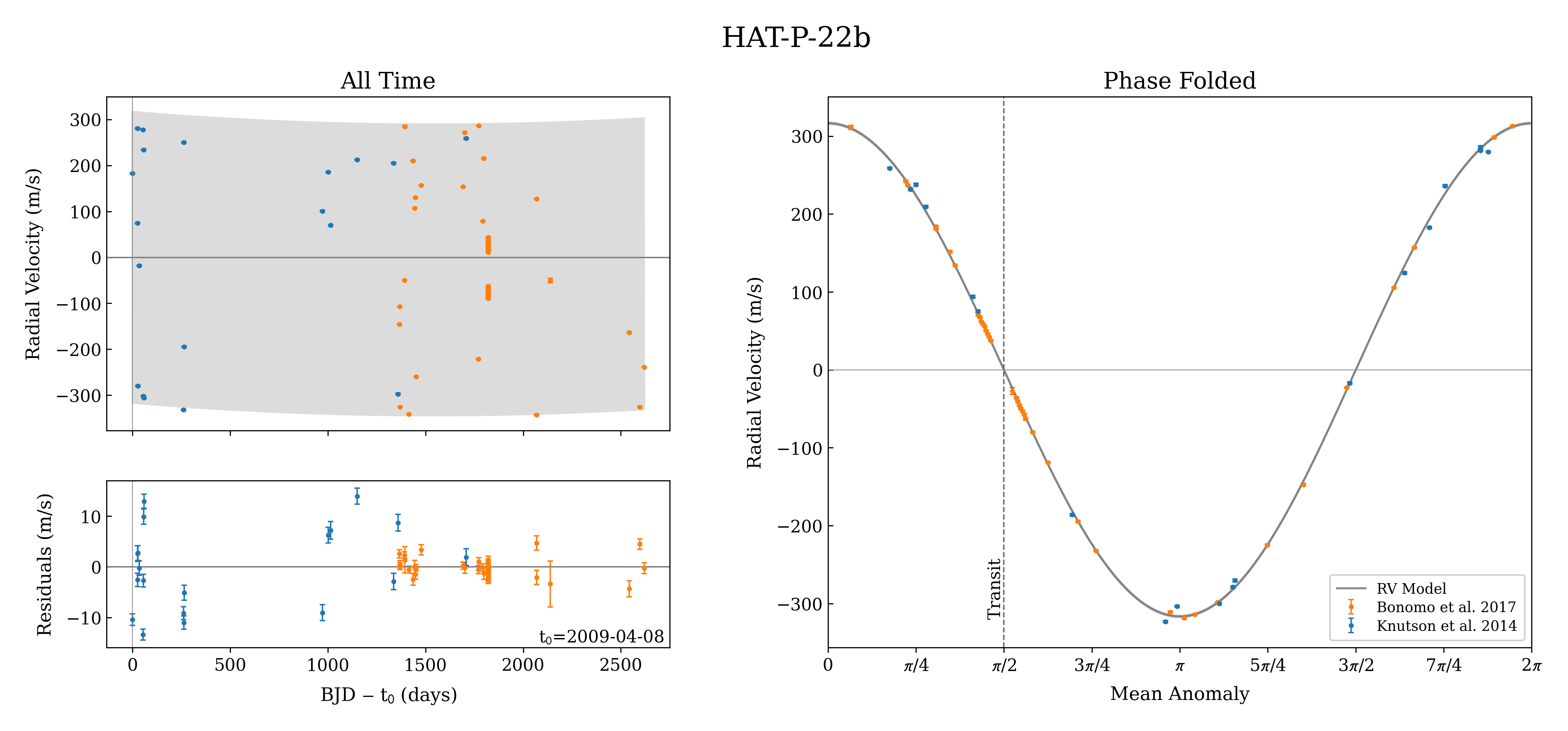
The following image displays the RV plot that is automatically generated during the model fit. It is saved in the file: examples/results/HAT-P-4/rv_fits/rv_constant_plot_linear.png.

Interpretation
Now that the model fitting is complete, we will use the Analyzer class to help interpret the results. Creating an instance of the Analyzer class requires the StarPlanet object and the results of a model fit. It is for this reason that we assigned the output of the model fits to the variables fit_circular, fit_eccentric, fit_linear, and fit_quadratic.
The following code snippet creates an Analyzer object with the results of the best model fit:
# create an ``Analyzer`` instance for the final fit results
analyzer = Analyzer(hatp4, fit_linear)
We can now call any relevant Analyzer methods, the result of which are written to the file: examples/results/HAT-P-4/analysis/rv_constant_analysis_linear.txt.
Model Comparison
Calling the model_comparison() method compares the model fits by calculating the Bayes factors and evaluating the strength of the evidence with thresholds given by Kass and Raftery [1995].
The following code snippet calls this method three times, once for each alternative model:
# compare the Bayesian evidence for the various model fits
analyzer.model_comparison(fit_circular)
analyzer.model_comparison(fit_eccentric)
analyzer.model_comparison(fit_quadratic)
Now the analysis file looks like this:
HAT-P-4b Analysis | model: 'rv_constant'

Model Comparison
---------------------------------------------------------------------------
 * Very strong evidence for Model 1 vs. Model 2  (B = 5.63e+04)
      Model 1: 'rv_constant_linear', logZ = -150.66
      Model 2: 'rv_constant_circular', logZ = -161.60

Model Comparison
---------------------------------------------------------------------------
 * Very strong evidence for Model 1 vs. Model 2  (B = 6.24e+04)
      Model 1: 'rv_constant_linear', logZ = -150.66
      Model 2: 'rv_constant_eccentric', logZ = -161.70

Model Comparison
---------------------------------------------------------------------------
 * Strong evidence for Model 1 vs. Model 2  (B = 4.32e+01)
      Model 1: 'rv_constant_linear', logZ = -150.66
      Model 2: 'rv_constant_quadratic', logZ = -154.42
This comparison confirms that there is strong evidence supporting the model of a circular orbit for HAT-P-4 b with a long-term linear trend.
Outer Companion Constraints
The final step of the HAT-P-4 analysis is to call the unknown_companion() method, which will use the best-fit results to constrain the mass and orbit of an outer companion that could induce the acceleration needed to account for the linear trend:
# investigate the trend as evidence of an outer companion planet
analyzer.unknown_companion()
This appends the following summary to the output file:
Unknown Companion Planet
---------------------------------------------------------------------------
 * Slope of the linear trend in the best-fit radial velocity model:
      dvdt = 2.24E-02 m/s/day
 * Minimum outer companion mass from slope (assuming P_min = 1.25 * baseline = 9.32 years):
      M_c > 2.27 M_jup
      a_c > 4.77 AU
      K_c > 30.51 m/s
 * Apparent orbital period derivative induced by the line-of-sight acceleration:
      dP/dt = 7.21E+00 ms/yr
The following table shows that these lower limits are consistent with the findings of Knutson et al. Upper limits cannot be determined from radial velocity data alone, and Knutson et al. performed additional analyses using AO imaging to address this limitation. The Bonomo et al. study did not report these constraints directly but instead referenced Knutson et al., stating that their best-fit parameters are in agreement.
Parameter |
Unit |
Knutson et al. [2014] |
OrbDot |
|---|---|---|---|
\(M_c\) |
\(M_\mathrm{Jup}\) |
\(1.5-310\) |
\(>2.3\) |
\(a_c\) |
\(\mathrm{AU}\) |
\(5-60\) |
\(>4.8\) |
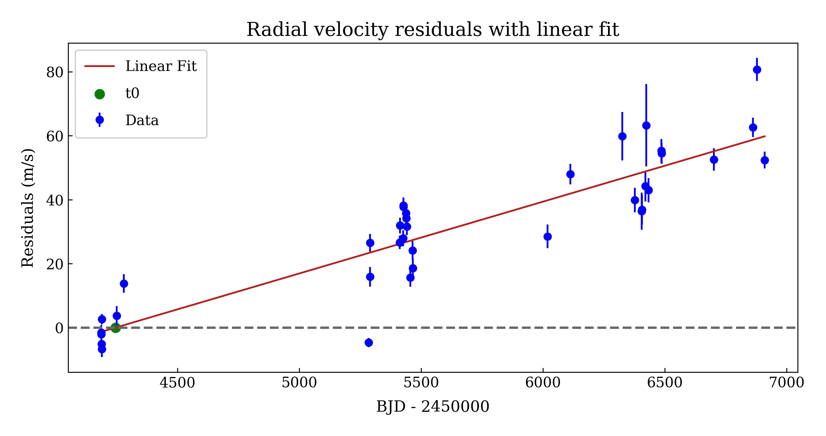
The following image displays a plot of the best-fit linear trend over the RV residuals, which is automatically generated by the unknown_companion() method.
HAT-P-22 b
We will now study the radial velocities of the Hot Jupiter host star HAT-P-22, for which Bonomo et al. found strong evidence of a long-term quadratic trend when combining their data with that of Knutson et al. At the time of the Knutson et al. study, the observational baseline was not long enough for them to detect curvature in the data.
As this analysis follows the same procedure as above, we will move through it quickly. Same as before, the first step is to create an instance of StarPlanet that represents HAT-P-22 b:
from orbdot.star_planet import StarPlanet
from orbdot.analysis import Analyzer

# initialize the StarPlanet class
hatp22 = StarPlanet('settings_files/HAT-P-22_settings.json')
Model Fits
The following code snippet fits the HAT-P-22 radial velocity data to the circular and eccentric orbit models, without including long-term trends (Models 1 and 2):
# run an RV model fit of a circular orbit
fit_circular = hatp22.run_rv_fit(['t0', 'P0', 'K', 'v0', 'jit'], file_suffix='_circular')

# run an RV model fit of an eccentric orbit
fit_eccentric = hatp22.run_rv_fit(['t0', 'P0', 'K', 'v0', 'jit', 'ecosw', 'esinw'], file_suffix='_eccentric')
Once the model fits are complete, the output files are found in the directory: examples/results/HAT-P-22/rv_fits/. The dropdown menus below show the contents of the *_summary.txt files, which provide a convenient summary of the results.
Summary of the HAT-P-22 circular orbit RV fit:
Stats
-----
Sampler: nestle
Free parameters: ['t0' 'P0' 'K' 'jit_Bon' 'jit_Knu' 'v0_Bon' 'v0_Knu']
log(Z) = -196.3 ± 0.13
Run time (s): 53.49
Num live points: 1000
Evidence tolerance: 0.01
Eff. samples per second: 124

Results
-------
t0 = 2454930.2209793446 + 0.0009148432873189449 - 0.0009883171878755093
P0 = 3.212228430587123 + 2.947214678084009e-06 - 2.9119439011182635e-06
K = 314.36239007855045 + 1.016465801944321 - 0.9944198208758621
jit_Bon = 3.3790987460139412 + 0.48360436956763175 - 0.4044244700780677
jit_Knu = 11.972129829710717 + 2.341468700814186 - 1.8093885079082543
v0_Bon = 12638.052030084446 + 0.6779472350772267 - 0.7051319365709787
v0_Knu = -40.90170211162001 + 2.7515356496278613 - 2.765810650957228

Fixed Parameters
----------------
e0 = 0.0
w0 = 0.0
dvdt = 0.0
ddvdt = 0.0
Summary of the HAT-P-22 eccentric orbit RV fit:
Stats
-----
Sampler: nestle
Free parameters: ['t0' 'P0' 'K' 'ecosw' 'esinw' 'jit_Bon' 'jit_Knu' 'v0_Bon' 'v0_Knu']
log(Z) = -199.54 ± 0.14
Run time (s): 80.45
Num live points: 1000
Evidence tolerance: 0.01
Eff. samples per second: 93

Results
-------
t0 = 2454930.2207814716 + 0.000935626681894064 - 0.0009516454301774502
P0 = 3.2122251871335674 + 5.658060811430943e-06 - 5.6578486766767355e-06
K = 314.12585629873524 + 1.0071310157063635 - 1.011800634438373
ecosw = 0.0023600533871185117 + 0.003617665664077273 - 0.0035947678543966524
esinw = 0.010264458739563949 + 0.005902351169264311 - 0.005683696346013998
jit_Bon = 3.229168546671116 + 0.4732269272279739 - 0.3893554633516727
jit_Knu = 12.344854539818977 + 2.4136363529357006 - 1.8935382244620147
v0_Bon = 12637.499340966315 + 0.8780776066996623 - 0.9067069574630295
v0_Knu = -41.35612623074179 + 2.9698691751275135 - 2.926142302027813
e (derived) = 0.010532282051210947 + 0.0058091004680366895 - 0.005597429099943213
w0 (derived) = 1.3447993835698682 + 0.3575276216655931 - 0.35392835006713863

Fixed Parameters
----------------
dvdt = 0.0
ddvdt = 0.0
The Bayesian evidence implies that the circular orbit model, with log(Z) = -196.3, is a better fit to the data than an eccentric orbit, which has log(Z) = -199.54. These findings agree with the results from the Bonomo et al. and Knutson et al. studies.
Next, we will focus on the circular orbit model for HAT-P-22 b, this time including the long-term linear and quadratic trends with the "dvdt" and "ddvdt" parameters (Models 3 and 4):
# run an RV model fit of a circular orbit with a linear trend
fit_linear = hatp22.run_rv_fit(['t0', 'P0', 'K', 'v0', 'jit', 'dvdt'], file_suffix='_linear')

# run an RV model fit of a circular orbit with a quadratic trend
fit_quadratic = hatp22.run_rv_fit(['t0', 'P0', 'K', 'v0', 'jit', 'dvdt', 'ddvdt'], file_suffix='_quadratic')
Summary of the HAT-P-22 linear trend RV fit:
Stats
-----
Sampler: nestle
Free parameters: ['t0' 'P0' 'K' 'dvdt' 'jit_Bon' 'jit_Knu' 'v0_Bon' 'v0_Knu']
log(Z) = -193.41 ± 0.14
Run time (s): 64.73
Num live points: 1000
Evidence tolerance: 0.01
Eff. samples per second: 109

Results
-------
t0 = 2454930.2210348514 + 0.0009558191522955894 - 0.0010035419836640358
P0 = 3.212229380385748 + 2.4844342401131314e-06 - 2.5362280267060555e-06
K = 315.1987432251591 + 0.784965083072052 - 0.779657635217859
dvdt = 0.006352346295932204 + 0.0014840271067953197 - 0.001566825201639855
jit_Bon = 2.4236899765310995 + 0.4011110829325548 - 0.32738639082012
jit_Knu = 14.84872017277269 + 3.092170355223981 - 2.354841306198354
v0_Bon = 12626.635056948253 + 2.864358835211533 - 2.7032946015388006
v0_Knu = -44.219049782421315 + 3.582727327111016 - 3.527302580555819

Fixed Parameters
----------------
e0 = 0.0
w0 = 0.0
ddvdt = 0.0
Summary of the HAT-P-22 quadratic trend RV fit:
Stats
-----
Sampler: nestle
Free parameters: ['t0' 'P0' 'K' 'dvdt' 'ddvdt' 'jit_Bon' 'jit_Knu' 'v0_Bon' 'v0_Knu']
log(Z) = -176.67 ± 0.17
Run time (s): 92.72
Num live points: 1000
Evidence tolerance: 0.01
Eff. samples per second: 81

Results
-------
t0 = 2454930.220904868 + 0.0009081698954105377 - 0.000938760582357645
P0 = 3.2122337625856625 + 2.1047943774554767e-06 - 2.0765374282305515e-06
K = 316.5092574320025 + 0.561605713510744 - 0.5529356624163029
dvdt = -0.03533039459243746 + 0.005307926327840582 - 0.005931347652372576
ddvdt = 2.2931992846055927e-05 + 3.1983652391035815e-06 - 2.8800379972539464e-06
jit_Bon = 1.4348768181376026 + 0.31369808335633564 - 0.2687117730446722
jit_Knu = 8.679671141065063 + 1.9024650861196513 - 1.4890214006954068
v0_Bon = 12662.751524196548 + 5.452072293634046 - 4.76741190116627
v0_Knu = -29.97713099689939 + 2.8625404047107033 - 2.73711899165702

Fixed Parameters
----------------
e0 = 0.0
w0 = 0.0
These results show that the quadratic trend model, with log(Z) = -176.67, is a far better fit to the data than the linear trend model, which has log(Z) = -193.41. The following table compares the OrbDot results for the quadratic model with those of Bonomo et al.:
Parameter |
Unit |
Bonomo et al. [2017] |
OrbDot |
|---|---|---|---|
\(K\) |
\(\mathrm{m \, s^{-1}}\) |
\(316.49 \pm 0.60\) |
\(316.51^{\,+0.56}_{\,-0.55}\) |
\(\dot{\gamma}\) |
\(\mathrm{m \, s^{-1} \, days^{-1}}\) |
\(-0.0328 \pm 0.0064\) |
\(-0.0353^{\,+0.0053}_{\,-0.0059}\) |
\(\ddot{\gamma}\) |
\(\mathrm{m \, s^{-1} \, days^{-2}}\) |
\(2.26 \times 10^{-5} \pm 0.30 \times 10^{-5}\) |
\(2.29 \times 10^{-5} \pm 0.32 \times 10^{-5}\) |
\(\sigma_{\mathrm{jitter}}\) |
\(\mathrm{m \, s^{-1}}\) |
\(1.15^{\,+0.32}_{\,-0.29}\) |
\(1.43^{\,+0.31}_{\,-0.27}\) |
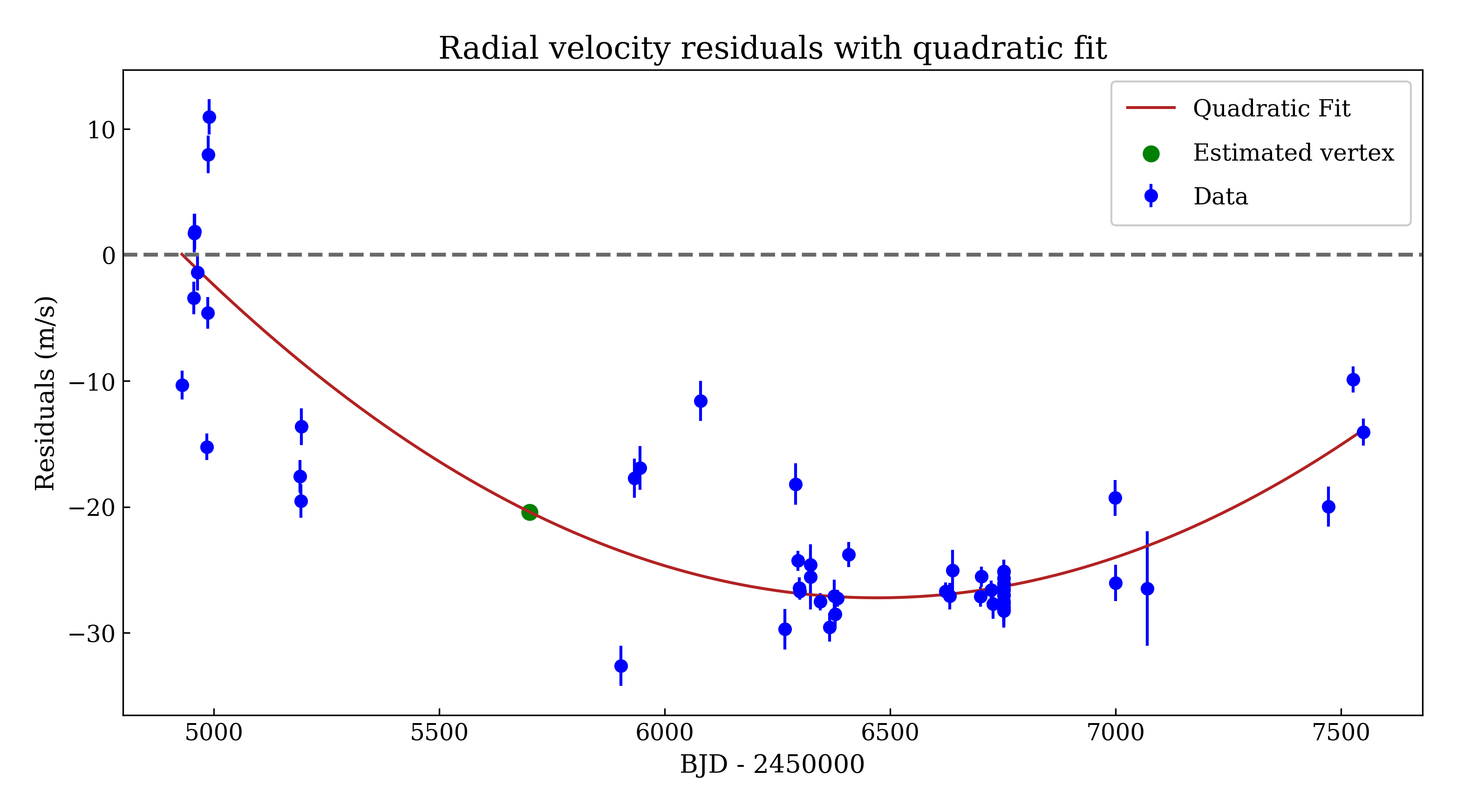
The following image displays the radial velocity plot, which is automatically generated during the model fit. It is saved in the file: examples/results/HAT-P-22/rv_fits/rv_constant_plot_quadratic.png.
Interpretation
Now that the model fitting is complete, we will use the Analyzer class to help interpret the results. The following code snippet creates an Analyzer object with the results of the quadratic trend fit:
# create an ``Analyzer`` instance for the final fit results
analyzer = Analyzer(hatp22, fit_quadratic)
We can now call any relevant Analyzer methods, the result of which will appear in the file: analysis/rv_constant_analysis_quadratic.txt.
Model Comparison
The following code snippet calls the model_comparison() method three times, once for each alternative model:
# compare the Bayesian evidence for the various model fits
analyzer.model_comparison(fit_circular)
analyzer.model_comparison(fit_eccentric)
analyzer.model_comparison(fit_linear)
Now the analysis file looks like this:
HAT-P-22b Analysis | model: 'rv_constant'

Model Comparison
---------------------------------------------------------------------------
 * Very strong evidence for Model 1 vs. Model 2  (B = 3.35e+08)
      Model 1: 'rv_constant_quadratic', logZ = -176.67
      Model 2: 'rv_constant_circular', logZ = -196.30

Model Comparison
---------------------------------------------------------------------------
 * Very strong evidence for Model 1 vs. Model 2  (B = 8.59e+09)
      Model 1: 'rv_constant_quadratic', logZ = -176.67
      Model 2: 'rv_constant_eccentric', logZ = -199.54

Model Comparison
---------------------------------------------------------------------------
 * Very strong evidence for Model 1 vs. Model 2  (B = 1.86e+07)
      Model 1: 'rv_constant_quadratic', logZ = -176.67
      Model 2: 'rv_constant_linear', logZ = -193.41
This comparison confirms that the evidence supporting the model of a circular orbit with a long-term quadratic trend is very strong.
Outer Companion Constraints
Finally, we again call the unknown_companion() method. This time, it will automatically detect that both the first and second-order acceleration terms are part of the model.
# investigate the trend as evidence of an outer companion planet
analyzer.unknown_companion()
This appends the following summary to the analysis/rv_constant_analysis_quadratic.txt file:
Unknown Companion Planet
---------------------------------------------------------------------------
 * Acceleration terms from the best-fit radial velocity model:
      linear: dvdt = -3.53E-02 m/s/day
      quadratic: ddvdt = 2.29E-05 m/s^2/day
 * Constraints on the mass and orbit of an outer companion from a quadratic RV:
      P_c > 20.25 years
      M_c > 2.87 M_jup
      a_c > 7.21 AU
      K_c > 31.77 m/s
The following table demonstrates that these values are in excellent agreement with the results from Bonomo et al.:
Parameter |
Unit |
Bonomo et al. [2017] |
OrbDot |
|---|---|---|---|
\(P_c\) |
\(\mathrm{days}\) |
\(>20.8\) |
\(>20.3\) |
\(M_c\sin{i_c}\) |
\(M_\mathrm{Jup}\) |
\(>3.0\) |
\(>2.9\) |
\(K_c\) |
\(\mathrm{m\,s^{-1}}\) |
\(>32.9\) |
\(>31.8\) |
The following image displays a plot of the best-fit quadratic trend over the RV residuals, which is automatically generated by the unknown_companion() method.