Theory
Model Parameters
It is important for the user to be familiar with the symbols and definitions of the OrbDot parameter set, listed in the table below. Some of these parameters are not currently implemented in the OrbDot models, but are planned for future integration. These are indicated with a footnote [*].
Orbital Elements
Note: the orbital elements are defined at time \(t=t_0\).
Parameter
OrbDot Symbol
Unit
Description
\(t_0\)
t0\(\mathrm{BJD}_\mathrm{TDB}\)
The reference transit mid-time.
\(P_0\)
P0\(\mathrm{days}\)
The observed orbital period.
\(e_0\)
e0The eccentricity of the orbit.
\(\omega_0\)
w0\(\mathrm{rad}\)
The argument of pericenter of the planetary orbit.
\(i_0\)
i0\(\mathrm{deg}\)
The line-of-sight inclination of the orbit.
\(\Omega_0\)
O0\(\mathrm{rad}\)
The longitude of the ascending node. [*]
Coupled Parameters
Parameter
OrbDot Symbol
Unit
Description
\(e_0 \cos{\omega_0}\)
ecoswThe eccentricity \(e_0\) multiplied by the cosine of \(\omega_0\).
\(e_0 \sin{\omega_0}\)
esinwThe eccentricity \(e_0\) multiplied by the sine of \(\omega_0\).
\(\sqrt{e_0}\,\cos{\omega_0}\)
sq_ecoswThe square root of \(e_0\) multiplied by the cosine of \(\omega_0\).
\(\sqrt{e_0}\,\sin{\omega_0}\)
sq_esinwThe square root of \(e_0\) multiplied by the sine of \(\omega_0\).
Time-Dependent Parameters
Parameter
OrbDot Symbol
Unit
Description
\(\frac{dP}{dE}\)
PdE\(\mathrm{days}\) \(E^{-1}\)
A constant change of the orbital period.
\(\frac{d \omega}{dE}\)
wdE\(\mathrm{rad}\) \(E^{-1}\)
A constant change of the argument of pericenter.
\(\frac{de}{dE}\)
edE\(E^{-1}\)
A constant change of the eccentricity. [*]_
\(\frac{di}{dE}\)
idE\(\mathrm{deg}\) \(E^{-1}\)
A constant change of the line-of-sight inclination. [*]_
\(\frac{d \Omega}{dE}\)
OdE\(\mathrm{rad}\) \(E^{-1}\)
A constant change of the long. of the ascending node. [*]_
Radial Velocity Parameters
Parameter
OrbDot Symbol
Unit
Description
\(K\)
Km \({\mathrm s}^{-1}\)
The radial velocity semi-amplitude.
\(\gamma_i\)
v0\(\mathrm{m}\) \({\mathrm s}^{-1}\)
The systemic radial velocity (instrument-dependant).
\(\sigma_j\)
jit\(\mathrm{m}\) \({\mathrm s}^{-1}\)
The “jitter” uncertainty term (instrument-dependant).
\(\dot{\gamma}\)
dvdt\(\mathrm{m}\) \({\mathrm s}^{-1}\) \({\mathrm{day}}^{-1}\)
A first-order acceleration term.
\(\ddot{\gamma}\)
ddvdt\(\mathrm{m}\) \({\mathrm s}^{-1}\) \({\mathrm{day}}^{-2}\)
A second-order acceleration term.
\(K_{\mathrm{tide}}\)
K_tide\(\mathrm{m}\) \({\mathrm s}^{-1}\)
The semi-amplitude of a stellar tidal radial velocity signal. [*]_
Coordinate System
The OrbDot models are defined for a coordinate system in which the sky plane lies on the x-z plane, and the y-axis points toward the observer along the line of sight.
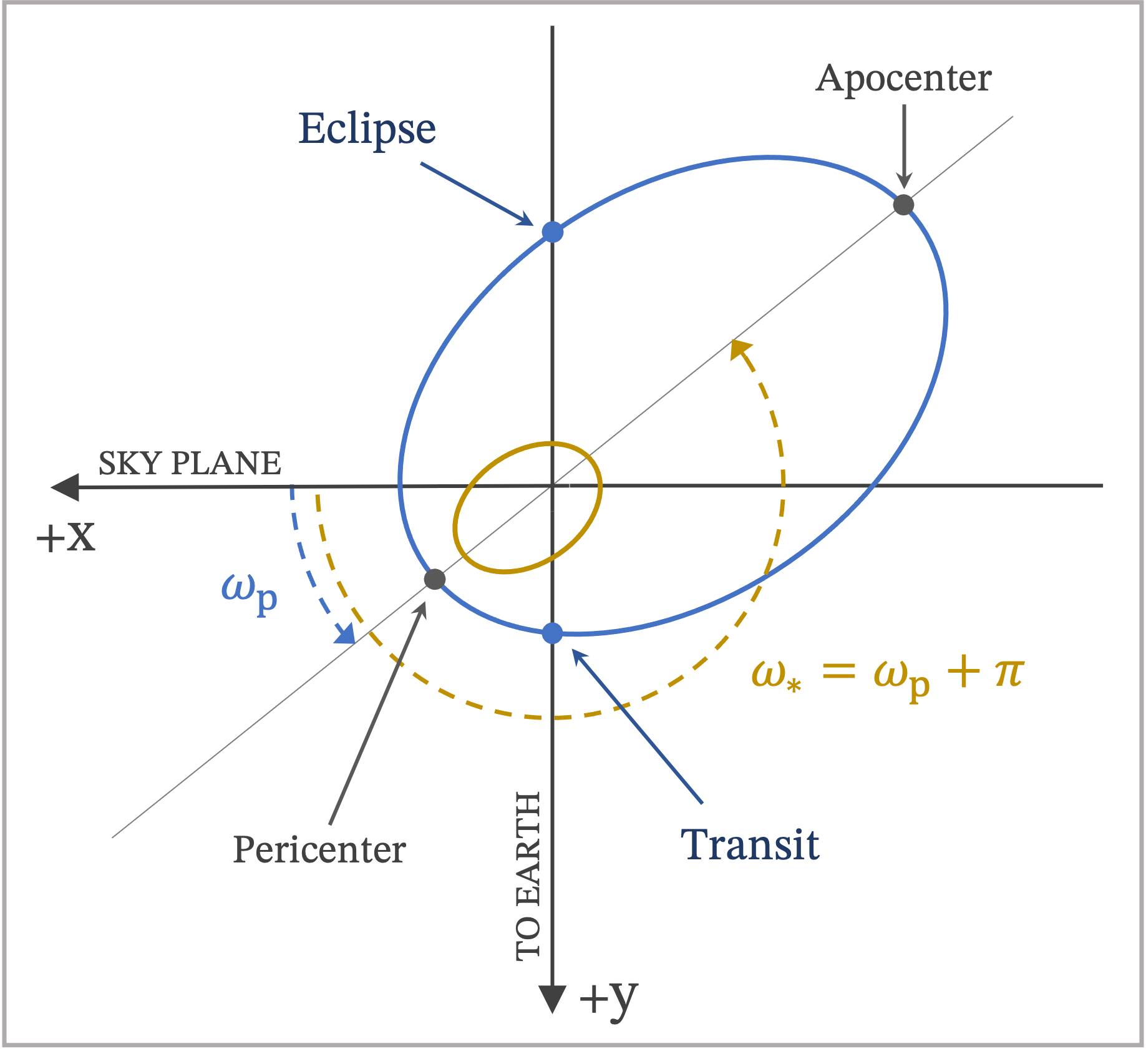
It is critical to maintain consistency in the definition of the argument of pericenter when simultaneously fitting transit mid-times, eclipse mid-times and radial velocities. In the OrbDot coordinate system, the argument of pericenter is measured from the positive x-axis, such that a transit occurs when the true anomaly \(\phi\) is equal to:
and an eclipse occurs when:
where \(\omega_p\) is the argument of pericenter of the planet’s orbit.
Transit and Eclipse Timing Models
OrbDot currently supports model fitting for three transit and eclipse timing models:
An unchanging orbit that is circular or eccentric, i.e. “constant-period”.
A constant evolution of the orbital period, i.e. “orbital decay”.
A constant evolution of the argument of pericenter, i.e. “apsidal precession”.
Constant-Period
For a planet on a circular, unchanging orbit, we expect a linear increase in the center times of both transits \(t_{\mathrm{I}}\) and eclipses \(t_{\mathrm{II}}\), modeled as:
where \(t_0\) is the reference transit time, \(P\) is the orbital period, and \(E\) is the epoch, which represents the number of orbits that have passed since time \(t_0\).
If the orbit is eccentric, an offset must be added to the eclipse times to account for the variable speed of the planet:
where \(\omega_p\) is the argument of pericenter of the planetary orbit and \(e\) is the eccentricity.
The orbdot.models.ttv_models.ttv_constant() method implements this model:
- orbdot.models.ttv_models.ttv_constant(t0, P0, e0, w0, E, primary=True)[source]
Constant-period model for transit and eclipse mid-times.
This method calculates the expected transit or eclipse mid-times for a single planet on an unchanging orbit.
- Parameters:
t0 (float) – Reference transit mid-time in \(\mathrm{BJD}_\mathrm{TDB}\).
P0 (float) – Orbital period in days.
e0 (float) – Eccentricity of the orbit.
w0 (float) – Argument of pericenter of the planetary orbit in radians.
E (array-like) – The epoch(s) at which to calculate the mid-times.
primary (bool, optional) – If True, returns the transit mid-time. If False, returns the eclipse mid-time. Default is True.
- Returns:
float or array-like – The predicted transit or eclipse times in \(\mathrm{BJD}_\mathrm{TDB}\).
Note
If the orbit is eccentric, an offset of \(\frac{2P}{\pi} e\cos{\omega}\) is added to the eclipse mid-times.
Orbital Decay
For a planet on a decaying circular orbit with a constant change of the orbital period, the mid-times of the transits \(t_{\mathrm{I}}\) and eclipses \(t_{\mathrm{II}}\) are modeled as:
where \(t_0\) is the reference transit time, \(P\) is the orbital period, \(dP/dE\) is the rate of change of the period in units of days per epoch, and \(E\) is the epoch. Though the main application of this model is for orbital decay, a positive period derivative is allowed.
The orbdot.models.ttv_models.ttv_decay() method implements this model:
- orbdot.models.ttv_models.ttv_decay(t0, P0, PdE, e0, w0, E, primary=True)[source]
Orbital decay model for transit and eclipse mid-times.
This method calculates the expected transit or eclipse mid-times for a single planet on an orbit with a constant change in the period. Though the main application of this model is for orbital decay, a positive period derivative is allowed.
- Parameters:
t0 (float) – Reference transit time in \(\mathrm{BJD}_\mathrm{TDB}\).
P0 (float) – Orbital period at the reference mid-time in days.
PdE (float) – Rate of change of the orbital period in days per epoch.
e0 (float) – Eccentricity of the orbit.
w0 (float) – Argument of pericenter of the planetary orbit in radians.
E (array-like) – The epoch(s) at which to calculate the mid-times.
primary (bool, optional) – If True, returns the transit mid-time. If False, returns the eclipse mid-time. Default is True.
- Returns:
float or array-like – The predicted transit or eclipse times in \(\mathrm{BJD}_\mathrm{TDB}\).
Note
If the orbit is eccentric, an offset of \(\frac{2P}{\pi} e\cos{\omega}\) is added to the eclipse mid-times.
Apsidal Precession
For a planet on an elliptical orbit undergoing apsidal precession, the mid-times of the transits \(t_{\mathrm{I}}\) and eclipses \(t_{\mathrm{II}}\) are modeled as [Giménez and Bastero, 1995, Patra et al., 2017]:
where \(t_0\) is the reference transit time, \(e\) is the orbit eccentricity, \(\omega_p\) is the argument of pericenter, and \(E\) is the epoch. We assume that \(\omega_p\) evolves at a constant rate, denoted as \(d\omega/dE\), such that at any given epoch \(\omega_p\) is given by:
where \(\omega_0\) is the value of \(\omega_p\) at time \(t_0\).
In the equations above, \(P_a\) represents the anomalistic orbital period, i.e. the elapsed time between subsequent pericenter passages, and \(P_s\) is the sidereal period, representing the observed orbital period of the system. These are related by:
The orbdot.models.ttv_models.ttv_precession method implements this model:
- orbdot.models.ttv_models.ttv_precession(t0, P0, e0, w0, wdE, E, primary=True)[source]
Apsidal precession model for transit and eclipse mid-times.
This method calculates the expected transit or eclipse mid-times for an elliptical orbit undergoing apsidal precession. It uses a numerical approximation for low eccentricities that is adapted from equation (15) in Giminez and Bastero (1995) [1]_ by Patra et al. (2017) [2]_.
- Parameters:
t0 (float) – Reference transit time in \(\mathrm{BJD}_\mathrm{TDB}\).
P0 (float) – The sidereal period in days.
e0 (float) – Eccentricity of the orbit.
w0 (float) – Argument of pericenter of the planetary orbit at the reference mid-time in radians.
wdE (float) – Apsidal precession rate in radians per epoch.
E (array-like) – The epoch(s) at which to calculate the mid-times.
primary (bool, optional) – If True, returns the transit mid-time. If False, returns the eclipse mid-time. Default is True.
- Returns:
float or array-like – The predicted transit or eclipse times in \(\mathrm{BJD}_\mathrm{TDB}\).
References
Radial Velocity Models
OrbDot currently supports model fitting for three radial velocity models:
An unchanging orbit that is circular or eccentric, i.e. “constant-period”.
A constant evolution of the orbital period, i.e. “orbital decay”.
A constant evolution of the argument of pericenter, i.e. “apsidal precession”.
Background
Many exoplanet host stars exhibit noticeable periodic radial velocity (RV) variations as they “wobble” around the center of mass of the star-planet system. The amplitude of this effect can be expressed as:
where \(M_p\) is the planet mass, \(M_{\star}\) is the star mass, \(i\) is the line-of-sight inclination of the orbit, and \(G\) is the universal gravitational constant.
At any given time, the star’s radial velocity depends on the planet’s position in its orbit, defined by the true anomaly \(\phi\), and the systemic velocity along the line-of-sight, denoted as \(\gamma\). When measurements from multiple instruments are combined, it is standard practice to fit the systemic velocity individually for each source to account for instrumental variations, denoted \(\gamma_i\).
The OrbDot radial velocity models also include first and second-order acceleration terms, \(\dot{\gamma}\) and \(\ddot{\gamma}\) respectively, to accommodate potential perturbations from an outer, non-resonant companion planet with an orbital period longer than the observational baseline. The total observed radial velocity signal is:
where \(\omega_p\) is the argument of pericenter of the planet’s orbit and \(t_0\) is the mid-time of a reference transit.
To avoid underestimating uncertainties, the radial velocity model fits include an instrument-dependant “jitter” parameter that represents systematic noise. When "jit" is given as a free parameter, it is added in quadrature with the individual measurement errors in the log-likelihood:
where \(\sigma_i\) is the measurement error and \(\sigma_{j}\) is the instrument-dependent jitter term.
Constant-Period
The orbdot.models.rv_models.rv_constant() method implements the constant-period radial velocity model:
- orbdot.models.rv_models.rv_constant(t0, P0, e0, w0, K, v0, dvdt, ddvdt, t)[source]
Constant-period model for radial velocities.
This method calculates the expected radial velocity signal of a star that hosts a planet on an unchanging orbit.
- Parameters:
t0 (float) – Reference transit mid-time in \(\mathrm{BJD}_\mathrm{TDB}\).
P0 (float) – The orbital period in days.
e0 (float) – Eccentricity of the orbit.
w0 (float) – Argument of pericenter of the planetary orbit in radians.
K (float) – Radial velocity semi-amplitude in m/s.
v0 (float) – Systemic radial velocity in m/s.
dvdt (float) – First-order acceleration term in m/s/day.
ddvdt (float) – Second-order acceleration term in m/s/day^2.
t (float) – Measurement time(s) in \(\mathrm{BJD}_\mathrm{TDB}\).
- Returns:
float or array-like – The expected radial velocity signal at the given time(s), including long-term trends.
Notes
Tip
In this model, the orbital elements do not evolve, which means that \(\omega_p=\omega_0\), \(e=e_0\), and \(P=P_0\).
The following steps outline the implementation of this method:
Calculate the true anomaly, eccentric anomaly, and mean anomaly at mid-transit.
In the OrbDot coordinate system, we know that the true anomaly at the transit center is:
\[\phi_0 = \frac{\pi}{2} - \omega_p\]where \(\omega_p\) is the argument of pericenter of the planetary orbit. The eccentric anomaly may then be calculated by:
\[\tan \left(\frac{\mathrm{E}_0}{2}\right) = \sqrt{\frac{1-e}{1+e}} \tan \left(\frac{\phi_0}{2}\right)\]which yields the mean anomaly via Kepler’s equation:
\[\mathrm{M}_0 = \mathrm{E}_0 - e \sin\mathrm{E}_0\]Determine the time of pericenter passage.
The time of pericenter passage \(t_p\) is related to the mean anomaly at \(t_0\) by:
\[\mathrm{M}_0 = n \left(t_0 - t_p\right)\]where \(n = 2 \pi/P\) is the mean motion.
Calculate the true anomaly of the planet at the given time.
With the time of pericenter passage, the planet’s mean anomaly may be calculated at any time \(t\):
\[\mathrm{M} = n \left(t - t_p\right)\]allowing for the eccentric anomaly to be determined by solving Kepler’s equation:
\[\mathrm{M} = \mathrm{E} - e \sin \mathrm{E}\]Finally, the true anomaly at time \(t\) is determined by:
\[\tan \left(\frac{\phi}{2}\right) = \sqrt{\frac{1+e}{1-e}} \tan \left(\frac{ \mathrm{E}}{2}\right)\]Return the total RV signal, including long-term trends.
Thus, the total radial velocity signal at time \(t\) is:
\[v_r = K[\cos{(\phi+\omega_p)}+e\cos{\omega_p}] + \gamma_i + \dot{\gamma} \left(t-t_0\right) + \frac{1}{2} \ddot{\gamma} \left(t-t_0\right)^2\]where \(K\) is the semi-amplitude of the planetary signal, \(\gamma_i\) is the systemic radial velocity, and \(\dot{ \gamma}\) and \(\ddot{\gamma}\) are first and second-order acceleration terms, respectively.
Orbital Decay
The orbdot.models.rv_models.rv_decay() method implements the orbital decay radial velocity model:
- orbdot.models.rv_models.rv_decay(t0, P0, e0, w0, K, v0, dvdt, ddvdt, PdE, t)[source]
Orbital decay model for radial velocities.
This method calculates the expected radial velocity signal of a star that hosts a planet on an orbit with a constant change in the period. Though the main application of this model is for orbital decay, a positive period derivative is allowed.
Note
This function assumes that the change in the RV semi-amplitude \(K\) is negligible.
- Parameters:
t0 (float) – Reference transit mid-time in \(\mathrm{BJD}_\mathrm{TDB}\).
P0 (float) – Orbital period at the reference mid-time, in days.
e0 (float) – Eccentricity of the orbit.
w0 (float) – Argument of pericenter of the planetary orbit in radians.
K (float) – Radial velocity semi-amplitude in m/s.
v0 (float) – Systemic radial velocity in m/s.
dvdt (float) – First-order acceleration term in m/s/day.
ddvdt (float) – Second-order acceleration term in m/s/day^2.
PdE (float) – Rate of change of the orbital period in days per epoch.
t (float) – Measurement time(s) in \(\mathrm{BJD}_\mathrm{TDB}\).
- Returns:
float or array-like – The expected radial velocity signal at the given time(s), including long-term trends.
Notes
Tip
In this model, the eccentricity and argument of pericenter do not evolve, which means that \(\omega_p=\omega_0\) and \(e=e_0\).
The following steps outline the implementation of this method:
Calculate the orbital period at the given time.
For a decaying orbit, the orbital period is dependant on time. Assuming that the rate-of-change is constant, the period at any epoch \(E\) is:
\[P\left(E\right) = P_0 + \frac{dP}{dE}\,E\]where \(E\) is determined by truncating the result of the following equation to an integer value:
\[E = \frac{(t - t_0)}{P_0}\]Calculate the latest time of pericenter passage.
As the orbit shrinks, the relative time of pericenter passage will evolve, so it must be calculated relative to the most recent transit mid-time:
\[t_{\mathrm{I}} = t_0 + PE + \frac{1}{2}\frac{dP}{dE}\,E^2\]In the OrbDot coordinate system, we know that the true anomaly at the transit center is:
\[\phi_{\mathrm{I}} = \frac{\pi}{2} - \omega_p\]The eccentric anomaly may then be calculated by:
\[\tan \left(\frac{\mathrm{E}_{\mathrm{I}}}{2}\right) = \sqrt{\frac{1-e}{ 1+e}}\tan \left( \frac{\phi_{\mathrm{I}}}{2}\right)\]which yields the mean anomaly via Kepler’s equation:
\[\mathrm{M}_{\mathrm{I}} = \mathrm{E}_{\mathrm{I}} - e \sin\mathrm{E}_{\mathrm{I}}\]Finally, the time of pericenter passage \(t_p\) is related to the mean anomaly by:
\[\mathrm{M}_{\mathrm{I}} = n \left(t_{\mathrm{I}} - t_p\right)\]where \(n = 2 \pi/P\) is the mean motion.
Calculate the true anomaly of the planet at the given time.
With the time of latest pericenter passage, the planet’s mean anomaly at time \(t\) may be calculated by:
\[\mathrm{M} = n \left(t - t_p\right)\]allowing for the eccentric anomaly to be determined by solving Kepler’s equation:
\[\mathrm{M} = \mathrm{E} - e \sin \mathrm{E}\]Finally, the true anomaly at time \(t\) is determined by:
\[\tan \left(\frac{\phi}{2}\right) = \sqrt{\frac{1+e}{1-e}} \tan \left(\frac{ \mathrm{E}}{2}\right)\]Return the total RV signal, including long-term trends.
Thus, the total radial velocity signal at time \(t\) is:
\[v_r = K[\cos{(\phi+\omega_p)}+e\cos{\omega_p}] + \gamma_i + \dot{\gamma} \left(t-t_0\right) + \frac{1}{2} \ddot{\gamma} \left(t-t_0\right)^2\]where \(K\) is the semi-amplitude of the planetary signal, \(\gamma_i\) is the systemic radial velocity, and \(\dot{ \gamma}\) and \(\ddot{\gamma}\) are first and second-order acceleration terms, respectively.
Apsidal Precession
The orbdot.models.rv_models.rv_precession() method implements the apsidal precession radial velocity model:
- orbdot.models.rv_models.rv_precession(t0, P0, e0, w0, K, v0, dvdt, ddvdt, wdE, t)[source]
Apsidal precession model for radial velocities.
This method calculates the expected radial velocity signal of a star that hosts a planet on an elliptical orbit undergoing apsidal precession.
- Parameters:
t0 (float) – Reference transit mid-time in \(\mathrm{BJD}_\mathrm{TDB}\).
P0 (float) – The sidereal period in days.
e0 (float) – Eccentricity of the orbit.
w0 (float) – Argument of pericenter of the planetary orbit at the reference mid-time, in radians.
K (float) – Radial velocity semi-amplitude in m/s.
v0 (float) – Systemic radial velocity in m/s.
dvdt (float) – First-order acceleration term in m/s/day.
ddvdt (float) – Second-order acceleration term in m/s/day^2.
wdE (float) – Apsidal precession rate in radians per epoch.
t (float) – Measurement time(s) in \(\mathrm{BJD}_\mathrm{TDB}\).
- Returns:
float or array-like – The expected radial velocity signal at the given time(s), including long-term trends.
Notes
Tip
In this model, the eccentricity and orbital period not evolve, which means that \(e=e_0\) and \(P_s=P_0\), where \(P_s\) is the sidereal period.
The following steps outline the implementation of this method:
Calculate the anomalistic period and argument of pericenter.
For a precessing orbit, there is a distinction between the sidereal (observed) orbital period \(P_s\) and the anomalistic orbital period \(P_a\). They are related by:
\[P_s = P_a\left(1-\frac{d\omega/{dE}}{2\pi}\right)\]where \(d\omega/{dE}\) is the apsidal precession rate in radians per epoch. The argument of pericenter of the planet’s orbit is a function of time, such that for any epoch \(E\) it is:
\[\omega_p\left(E\right) = \omega_0 + \frac{d\omega}{dE}\,E.\]where \(E\) is determined by truncating the result of the following equation to an integer value:
\[E = \frac{(t - t_0)}{P_s}\]Calculate the latest time of pericenter passage.
As the orbit is precessing, the time of pericenter passage must be calculated relative to the most recent transit mid-time:
\[t_{\mathrm{I}} = t_0 + P_s E - \frac{e P_a}{\pi}\cos{\omega_p}\]In the OrbDot coordinate system, we know that the true anomaly at the transit center is:
\[\phi_{\mathrm{I}} = \frac{\pi}{2} - \omega_p\left(E\right)\]The eccentric anomaly may then be calculated by:
\[\tan\left(\frac{\mathrm{E}_{\mathrm{I}}}{2}\right) = \sqrt{\frac{1-e}{1+e}} \tan\left(\frac{\phi_{\mathrm{I}}}{2}\right)\]which yields the mean anomaly via Kepler’s equation:
\[\mathrm{M}_{\mathrm{I}} = \mathrm{E}_{\mathrm{I}} - e \sin\mathrm{E}_{\mathrm{I}}\]Finally, the time of pericenter passage \(t_p\) is related to the mean anomaly by:
\[\mathrm{M}_{\mathrm{I}} = n \left(t_{\mathrm{I}} - t_p\right)\]where \(n = 2 \pi/P_a\) is the mean motion.
Calculate the true anomaly of the planet at the given time.
With the time of latest pericenter passage, the planet’s mean anomaly at time \(t\) may be calculated by:
\[\mathrm{M} = n \left(t - t_p\right)\]allowing for the eccentric anomaly to be determined by solving Kepler’s equation:
\[\mathrm{M} = \mathrm{E} - e \sin \mathrm{E}\]Finally, the true anomaly at time \(t\) is determined by:
\[\tan \left(\frac{\phi}{2}\right) = \sqrt{\frac{1+e}{1-e}} \tan \left(\frac{ \mathrm{E}}{2}\right)\]Return the total RV signal, including long-term trends.
Thus, the total radial velocity signal at time \(t\) is:
\[v_r = K[\cos{(\phi+\omega_p)}+e\cos{\omega_p}] + \gamma_i + \dot{\gamma} \left(t-t_0\right) + \frac{1}{2} \ddot{\gamma} \left(t-t_0\right)^2\]where,
\[\omega_p\left(E\right) = w_0 + \frac{d\omega}{dE}\,E\]and where \(K\) is the semi-amplitude of the planetary signal, \(\gamma_i\) is the systemic radial velocity, and \(\dot{ \gamma}\) and \(\ddot{\gamma}\) are first and second-order acceleration terms, respectively.
Transit Duration Models
Attention
The transit duration features of OrbDot have not been thoroughly tested and validated at this time. The methods are available to use, but the results should be treated with caution until this notice is removed.
OrbDot currently supports model fitting for three transit duration models:
An unchanging orbit that is circular or eccentric, i.e. “constant-period”.
A constant evolution of the orbital period, i.e. “orbital decay”.
A constant evolution of the argument of pericenter, i.e. “apsidal precession”.
Constant-Period
In general, the transit duration \(T\) is calculated using equation (15) from Kipping [2010]:
where \(P\) is the orbital period, \(e\) is the orbit eccentricity, \(i\) is the line-of-sight inclination of the orbit, \(a_R\) is the semi major axis in units of stellar radii, and \(\varrho_c\) is the star-planet separation at mid-transit.
The orbdot.models.tdv_models.tdv_constant() method implements the constant-period transit duration model:
- orbdot.models.tdv_models.tdv_constant(P0, e0, w0, i0, E, M_s, R_s)[source]
Constant-period model for transit durations.
This method returns the expected transit duration for a single planet on an unchanging orbit using the
transit_durationmethod defined in this module.- Parameters:
P0 (float) – Orbital period in days.
e0 (float) – Eccentricity of the orbit.
w0 (float) – Argument of pericenter of the planetary orbit in radians.
i0 (float) – Line-of-sight inclination of the orbit in degrees.
E (array-like) – The epoch(s) at which to calculate the transit duration.
M_s (float) – Host star mass in solar masses.
R_s (float) – Host star radius in solar radii.
- Returns:
array-like – The predicted transit durations in minutes.
Orbital Decay
For a planet on a decaying orbit, the change in transit duration over time is captured by equation (58) from Kipping [2010]:
where \(\frac{dT}{da}\) is the change in the transit duration with changing semi-major axis and \(b\) is the impact parameter. In this case, the change in the transit duration per epoch may be expressed as:
such that the transit duration as a function of epoch \(E\) is:
The orbdot.models.tdv_models.tdv_decay() method implements the orbital decay transit duration model:
- orbdot.models.tdv_models.tdv_decay(P0, e0, w0, i0, PdE, E, M_s, R_s)[source]
Orbital decay model for transit durations.
This method calculates the expected transit duration for a single planet on an orbit with a constant change in the period, using Equation 58 from Kipping (2010) [1]_. Though the main application of this model is for orbital decay, a positive period derivative is allowed.
- Parameters:
P0 (float) – Orbital period at the reference mid-time in days.
e0 (float) – Eccentricity of the orbit.
w0 (float) – Argument of pericenter of the planetary orbit in radians.
i0 (float) – Line-of-sight inclination of the orbit in degrees.
PdE (float) – Rate of change of the orbital period in days per epoch.
E (array-like) – The epoch(s) at which to calculate the transit duration.
M_s (float) – Host star mass in solar masses.
R_s (float) – Host star radius in solar radii.
- Returns:
array-like – The predicted transit durations in minutes.
References
Apsidal Precession
For a planet on an elliptical orbit undergoing apsidal precession, the change in the argument of pericenter \(\omega_p\) affects the transit duration. This relationship is captured by equation (54) from Kipping [2010]:
where \(\frac{dT}{d \omega}\) is the change in the transit duration with changing argument of pericenter and \(b\) is the impact parameter. The change in the transit duration per epoch may be expressed as:
such that the transit duration as a function of epoch \(E\) is:
The orbdot.models.tdv_models.tdv_precession() method implements the apsidal precession transit duration model:
- orbdot.models.tdv_models.tdv_precession(P0, e0, w0, i0, wdE, E, M_s, R_s)[source]
Apsidal precession model for transit durations.
This method calculates the expected transit duration at the given epoch(s) for a single planet on an elliptical orbit undergoing apsidal precession, using Equation 54 from Kipping (2010) [1]_.
- Parameters:
P0 (float) – Orbital period in days.
e0 (float) – Eccentricity of the orbit.
w0 (float) – Argument of pericenter of the planetary orbit at the reference mid-time in radians.
i0 (float) – Line-of-sight inclination of the orbit in degrees.
wdE (float) – Apsidal precession rate in radians per epoch.
E (array-like) – The epoch(s) at which to calculate the transit duration.
M_s (float) – Host star mass in solar masses.
R_s (float) – Host star radius in solar radii.
- Returns:
array-like – The predicted transit durations in minutes.
References
The theory Module
The theory module provides several analytical models for investigating long-term variations in planetary orbits and their causes, many of which are used in the Analyzer class (see Interpreting the Results). The key methods of this class are listed below, organized by subject.
Equilibrium Tides
In the classical framework of equilibrium tides developed by Darwin [1908], orbital decay occurs when a planet’s orbital rate is faster than the rate of the host star’s rotation. The planet’s orbit could also be retrograde. This causes the star’s tidal bulge to lag behind the planet in its orbit, generating a net torque that transfers angular momentum from the planet’s orbit to the star’s spin. Moreover, energy stored within the tidal bulges is dissipated in one or both of the bodies through internal processes. Together, these effects lead to changes in the planet’s orbit, as well as the spins of the star and planet.
In practice, the tidal decay rate is characterized by the tidal energy dissipation rate into the star, and if the planet remains in a non-synchronous rotation state, within the planet as well. The efficiency of this energy loss is typically quantified by the tidal quality factor, \(Q\), which is inversely proportional to the energy lost per cycle [Goldreich and Soter, 1966]. A lower \(Q\) value corresponds to more efficient energy dissipation and, consequently, faster orbital decay. An even more useful parameter, used in the methods below, is the “modified” quality factor, \(Q^{'} = \frac{3}{2} \frac{Q}{k_2}\), which incorporates the second-order Love number of the body, \(k_2\).
The tidal evolution models implemented in OrbDot follow the constant time lag (or “viscous”) equilibrium tide approach (e.g., Correia and Laskar [2010], Hut [1981], Leconte et al. [2010], Levrard et al. [2007]) and are exact for any eccentricity, obliquity, or rotation rate. The following OrbDot functions are relevant to these effects:
- orbdot.models.theory.decay_star_pdot_from_quality_factor(P, e, M_s, M_p, R_s, Q_star, epsilon_s=0.0, P_rot_s=None)[source]
Calculate the rate of orbital decay driven by equilibrium tides in the host star.
This method computes the orbital decay rate for a given “modified” stellar tidal quality factor and, optionally, the host star’s rotation period and/or obliquity.
- Parameters:
P (float) – The orbital period in days.
e (float) – The eccentricity of the orbit.
M_s (float) – Host star mass in solar masses.
M_p (float) – Planet mass in earth masses.
R_s (float) – Host star radius in solar radii.
Q_star (float) – The host star’s modified annual tidal quality factor.
epsilon_s (float, optional) – Host star obliquity in degrees. Default is zero.
P_rot_s (float, optional) – Host star rotation period in days.
- Returns:
float – Orbital decay rate in days per epoch.
Notes
If equilibrium tides are the dominant driver of orbital evolution, the rate of orbital period decay due to stellar tides is given by:
\[\frac{dP}{dt}_{\mathrm{(star)}} = -\frac{27\pi}{Q_\star^{'}} \left(\frac{M_p}{ M_\star}\right) \left(\frac{R_\star}{a}\right)^5 \times \left[f(e) - g(e) \cos{ \varepsilon_\star} \frac{\dot{\theta}_\star}{n}\right]\]where \(Q_\star^{'}\) is the modified annual tidal quality factor of the star, \(\varepsilon_\star\) is the stellar obliquity (defined as the angle between the spin and orbital angular momentum vectors), \(\dot{\theta}_\star\) is the stellar spin frequency, \(n\) is the orbital mean motion, \(a\) is the semi major axis, \(M_p\) is the planet mass, \(M_\star\) is the stellar mass, and \(R_\star\) is the stellar radius. The eccentricity-dependent functions \(f(e)\) and \(g(e)\) are defined in the
decay_get_f_e()anddecay_get_g_e()methods.This equation is derived using Equations (2), (5), and (19) from [1]_ and is valid for any value of \(\dot{\theta}_\star\), \(\varepsilon_\star\), and \(e\). We see that if \(e=0\) and \(\varepsilon_\star=0\), the expression simplifies to:
\[\frac{dP}{dt}_{\mathrm{(star)}} = -\frac{27\pi}{Q_\star^{'}} \left(\frac{M_p}{ M_\star}\right) \left(\frac{R_\star}{a}\right)^5 \left[1 - \frac{\dot{ \theta}_\star}{n}\right]\]If the rotation rate of the star is unknown, it is assumed that \(\dot{\theta}_\star \ll n\), in which case the bracketed term approaches unity, leaving:
\[\frac{dP}{dt}_{\mathrm{(star)}} = -\frac{27\pi}{Q_\star^{'}} \left(\frac{M_p}{ M_\star}\right) \left(\frac{R_\star}{a}\right)^5\]References
- orbdot.models.theory.decay_star_quality_factor_from_pdot(P, e, M_s, M_p, R_s, dPdE, epsilon_s=0.0, P_rot_s=None)[source]
Calculate the host star’s modified stellar quality factor given an orbital decay rate.
Given an orbital decay rate and, optionally, the host star’s rotation period and obliquity, this method returns the host star’s modified tidal quality factor under the assumption that the decay is driven by equilibrium tides in the host star. See the
decay_star_pdot_from_quality_factor()docstring for a more detailed description of the relevant equations.- Parameters:
P (float) – The orbital period in days.
e (float) – The eccentricity of the orbit.
M_s (float) – Host star mass in solar masses.
M_p (float) – Planet mass in earth masses.
R_s (float) – Host star radius in solar radii.
dPdE (float) – Orbital decay rate in days per epoch.
epsilon_s (float, optional) – Host star obliquity in degrees. Default is zero.
P_rot_s (float, optional) – Host star rotation period in days.
- Returns:
float – The host star’s modified annual tidal quality factor.
- orbdot.models.theory.decay_planet_pdot_from_quality_factor(P, e, M_s, M_p, R_p, Q_planet, epsilon_p=0.0, P_rot_p=None)[source]
Calculate the rate of orbital decay driven by equilibrium tides in the planet.
This method computes the orbital decay rate for a given “modified” planetary tidal quality factor and, optionally, the planet’s rotation period and obliquity. This expression accounts for both eccentricity-driven and obliquity-driven tidal dissipation, providing a unified treatment of planetary tides.
- Parameters:
P (float) – The orbital period in days.
e (float) – The eccentricity of the orbit.
M_s (float) – Host star mass in solar masses.
M_p (float) – Planet mass in earth masses.
R_p (float) – Planet radius in earth radii.
Q_planet (float) – The planet’s modified annual tidal quality factor.
epsilon_p (float, optional) – Planetary obliquity in degrees. Default is zero.
P_rot_p (float, optional) – Planet rotation period in days.
- Returns:
float – Orbital decay rate in days per epoch.
Notes
If equilibrium tides are the dominant driver of orbital evolution, the rate of orbital period decay due to planetary tides is given by:
\[\frac{dP}{dt}_{\mathrm{(planet)}} = -\frac{27\pi}{Q_p^{'}} \left(\frac{M_\star}{ M_p}\right) \left(\frac{R_p}{a}\right)^5 \left[f(e) - g(e) \cos{\varepsilon_p} \frac{\dot{\theta}_p}{n}\right]\]where \(Q_p^{'}\) is the modified annual tidal quality factor of the planet, \(\varepsilon_p\) is the planetary obliquity (defined as the angle between the planet’s spin and orbital angular momentum vectors), \(\dot{\theta}_p\) is the planet’s spin frequency, \(n\) is the orbital mean motion, \(a\) is the semi major axis, \(M_p\) is the planet mass, \(M_\star\) is the stellar mass, and \(R_p\) is the planet’s radius. The eccentricity-dependent functions \(f(e)\) and \(g(e)\) are defined in the
decay_get_f_e()anddecay_get_g_e()methods.This equation is derived using Equations (2), (5), and (19) from [1]_ and is valid for any value of \(\dot{\theta}_p\), \(\varepsilon_p\), and \(e\).
If a rotation period is not provided, the planet’s spin frequency is calculated using the tidally-evolved equilibrium rate defined in
decay_get_equilibrium_spin_freq(), which is dependent on the eccentricity and planetary obliquity. In this case, the above equation can be expressed as:\[\frac{dP}{dt}_{\mathrm{(planet)}} = -\frac{27\pi}{Q_p^{'}} \left(\frac{M_\star}{ M_p}\right) \left(\frac{R_p}{a}\right)^5 \times \left[f(e) - \frac{g^2(e)}{h( e)}\frac{2 \cos^2{\varepsilon_p}}{(1 + \cos^2{\varepsilon_p})}\right]\]We see that if the orbit is circular and aligned, meaning \(e=0\) and \(\varepsilon_p=0\), the planetary contribution to orbital decay vanishes. In this case, the functions \(f(e)\), \(g(e)\), and \(h(e)\) approach unity, and the equilibrium spin rate synchronizes with the mean motion, \(\dot{\theta}_p=n\), leading to no net tidal energy dissipation in the planet.
- orbdot.models.theory.decay_planet_quality_factor_from_pdot(P, e, M_s, M_p, R_p, dPdE, epsilon_p=0.0, P_rot_p=None)[source]
Calculate the planet’s modified planetary quality factor given an orbital decay rate.
Given an orbital decay rate and, optionally, the planet’s rotation period and obliquity, this method returns the planet’s modified tidal quality factor under the assumption that the decay is driven by equilibrium tides in the planet. See the
decay_planet_pdot_from_quality_factor()docstring for a more detailed description of the relevant equations.- Parameters:
P (float) – The orbital period in days.
e (float) – The eccentricity of the orbit.
M_s (float) – Host star mass in solar masses.
M_p (float) – Planet mass in earth masses.
R_p (float) – Planet radius in earth radii.
dPdE (float) – Orbital decay rate in days per epoch.
epsilon_p (float, optional) – Planetary obliquity in degrees. Default is zero.
P_rot_p (float, optional) – Planet rotation period in days.
- Returns:
float – The planet’s modified annual tidal quality factor.
Notes
If a rotation period not provided for the planet, the planet’s spin frequency is calculated with the
decay_get_equilibrium_spin_freq()method.
- orbdot.models.theory.decay_empirical_quality_factor(P_orb, P_rot_s)[source]
Calculate the modified stellar tidal quality factor from an empirical law.
This method calculates the tidal forcing period of a star-planet system and uses it to estimate the star’s modified tidal quality factor with an empirical law derived by Penev et al. (2018) [1]_.
- Parameters:
P_orb (float) – Orbital period in days.
P_rot_s (float) – Period of the host star’s rotation in days.
- Returns:
tuple – The star’s modified tidal quality factor and the tidal forcing period of the system in days.
Notes
The “modified” tidal quality factor is a typical parameterization of the efficiency of tidal energy dissipation within a body. It is defined as:
\[Q_\star^{'} = \frac{3}{2} \frac{Q_\star}{k_{2,\star}}\]where \(Q_\star\) is the tidal quality factor and \(k_{2,\star}\) is the second-order potential Love number. The theoretical upper limit is \(k_{2,\star}=3/2\), that of a uniform density sphere, in which case \(Q_\star^{'} = Q_\star\).
This method estimates a value for \(Q_\star^{'}\) using an empirical law derived by Penev et al. (2018) [1]_:
\[Q^{'}_\star = \max\left(\frac{10^6}{(P_{\mathrm{tide}}/\mathrm{day})^{3.1}}, \, 10^5\right)\]where \(P_{\mathrm{tide}}\) is the tidal forcing period of the system, defined as:
\[P_{\mathrm{tide}} = \frac{1}{2\left(P_{\mathrm{orb}}^{-1} - P_{\mathrm{rot}}^{ -1}\right)}\]where \(P_{\mathrm{orb}}\) is the planet’s orbital period and \(P_{\mathrm{rot}}\) is the rotational period of the host star.
References
- orbdot.models.theory.decay_timescale(P, dPdE)[source]
Calculate the remaining lifetime of a planet on a decaying orbit.
- Parameters:
P (float) – Orbital period in days.
dPdE (float) – Orbital decay rate in days per epoch.
- Returns:
float – The remaining lifetime in millions of years (Myr).
Notes
For a planet on a decaying orbit, its remaining lifetime can be estimated as simply:
\[\tau = \frac{P_0}{|\dot{P}_{\mathrm{decay}}|}\]where \(\dot{P}_{\mathrm{decay}}\) is the orbital decay rate, and \(P_0\) is the observed orbital period.
- orbdot.models.theory.decay_energy_loss(P, dPdE, M_s, M_p)[source]
Calculate the rate of orbit energy loss due to tidal forces causing orbital decay.
This function uses Equation (9) from Yee et al. (2020) [1]_ to compute the rate at which the energy of a planetary orbit decreases as it decays due to tidal forces.
- Parameters:
P (float) – Orbital period in days.
dPdE (float) – Orbital decay rate in days per epoch.
M_s (float) – Mass of the host star in solar masses.
M_p (float) – Mass of the planet in earth masses.
- Returns:
float – The rate of orbital energy loss in watts.
Notes
As a planet’s orbit decays, the orbital energy and angular momentum will decrease over time. Equation (9) of Yee et al. (2020) [1]_ defines the rate of orbital energy loss as:
\[\frac{dE}{dt} = \frac{(2\pi)^{2/3} M_{\mathrm{p}}}{3} \left(\frac{G M_{\star}}{ P}\right)^{2/3} \frac{1}{P} \frac{dP}{dt}\]where \(G\) is the gravitational constant, \(M_{\star}\) is the host star mass, \(M_{\mathrm{p}}\) is the planet mass, \(P\) is the orbital period, and \(\frac{dP}{dt}\) is the orbital decay rate.
References
- orbdot.models.theory.decay_angular_momentum_loss(P, dPdE, M_s, M_p)[source]
Calculate the rate of angular momentum loss due to tidal forces causing orbital decay.
This function uses Equation (10) from Yee et al. (2020) [1]_ to compute the rate at which the angular momentum of a planetary orbit decreases as it decays due to tidal forces.
- Parameters:
P (float) – Orbital period in days.
dPdE (float) – Orbital decay rate in days per epoch.
M_s (float) – Host star mass in solar masses.
M_p (float) – Planet mass in earth masses.
- Returns:
float – The rate of orbital angular momentum loss in kg m^2 / s^2.
Notes
As a planet’s orbit decays, the orbital energy and angular momentum will decrease over time. Equation (10) of Yee et al. (2020) [1]_ defines the rate of orbital angular momentum loss as:
\[\frac{dL}{dt} = \frac{M_{\mathrm{p}}}{3(2\pi)^{1/3}} \left(\frac{G M_{\star}}{ P}\right)^{2/3} \frac{dP}{dt}\]where \(G\) is the gravitational constant, \(M_{\star}\) is the host star mass, \(M_{\mathrm{p}}\) is the planet mass, \(P\) is the orbital period, and \(\frac{dP}{dt}\) is the orbital decay rate.
References
Apsidal Precession
Apsidal precession is the gradual increase of the argument of pericenter of a planet’s orbit \(\omega_p\), meaning the line that connects the pericenter and apocenter of the orbit rotates through \(2\pi\) in one precession period. This effect may result from several factors, including general relativistic effects, perturbations from other planets, and gravitational moments arising from both the host star’s rotation and planetary tidal bulges.
The following OrbDot functions are relevant to these effects:
General Relativity
- orbdot.models.theory.precession_gr(P, e, M_s)[source]
Calculate the rate of apsidal precession predicted by general relativity.
This method returns the expected apsidal precession rate of the planet’s orbit due to general relativistic (GR) effects, using Equation (12) from Ragozzine and Wolf (2009) [1]_.
- Parameters:
P (float) – The orbital period in days.
e (float) – The eccentricity of the orbit.
M_s (float) – The host star mass in solar masses.
- Returns:
float – The precession rate in radians per epoch.
Notes
This method applies the lowest order of the relativistic contribution to apsidal precession, given in Equation (12) of Ragozzine and Wolf (2009) [1]_ as:
\[\dot{\omega}_{\mathrm{GR}} = \frac{3 G M_{\star} n}{a c^2(1 - e^2)}\]where \(G\) is the gravitational constant, \(c\) is the speed of light in a vacuum, \(M_{\star}\) is the host star mass, \(a\) is the planet’s semi major axis, \(e\) is the eccentricity, and \(n = 2\pi/P\) is the mean motion.
References
Rotation
- orbdot.models.theory.precession_rotational_planet(P, e, M_s, M_p, R_p, k2_p, P_rot_p)[source]
Calculates the rate of apsidal precession driven by planetary rotation.
This method returns the expected apsidal precession rate of a planet’s orbit due to its rotational bulge, calculated using Equations (10) and (11) from Ragozzine and Wolf (2009) [1]_.
- Parameters:
P (float) – The orbital period in days.
e (float) – The eccentricity of the orbit.
M_s (float) – The host star mass in solar masses.
M_p (float) – The planet mass in earth masses.
R_p (float) – The planet radius in earth radii.
k2_p (float) – The planet’s Love number.
P_rot_p (float) – The period of the planet’s rotation in days.
- Returns:
float – The precession rate in radians per epoch.
Notes
The rotation of a fluid body raises an oblate distortion (i.e., flattening) that perturbs the gravitational potential, driving apsidal precession. The rate of the apsidal precession induced by a planet’s rotational bulge is given in Equation (10) of Ragozzine and Wolf (2009) [1]_ as:
\[\dot{\omega}_{\mathrm{rot,p}} = \frac{n {R_p}^5 k_{2,p} {\dot{\theta}_p}^2}{2 a^2 G M_p} g_2(e)\]where \(\dot{\theta}_p\) is the rotational velocity of the planet, \(k_{2,p}\) is its second-order potential Love number, \(G\) is the gravitational constant, \(n = 2\pi/P\) is the orbit mean motion, \(a\) is the semi major axis, and \(M_p\) and \(R_p\) are the planet mass and radius, respectively.
The function \(g_2(e)\) represents an expansion in eccentricity \(e\), defined in Equation (11) of Ragozzine and Wolf (2009) [1]_ as:
\[g_2(e) = (1-e^2)^{-2}\]References
- orbdot.models.theory.precession_rotational_planet_k2(P, e, M_s, M_p, R_p, P_rot_p, dwdE)[source]
Calculate the Love number given a rate of apsidal precession driven by planetary rotation.
Given an apsidal precession rate for a planetary orbit, this method returns the second-order potential Love number of the planet \(k_{2,p}\) under the assumption that the precession is driven entirely by the rotational bulge of the planet. See the
precession_rotational_planet()docstring for a more detailed description of the relevant equations, which are adopted from Ragozzine and Wolf (2009) [1]_.- Parameters:
P (float) – The orbital period in days.
e (float) – The eccentricity of the orbit.
M_s (float) – The host star mass in solar masses.
M_p (float) – The planet mass in earth masses.
R_p (float) – The planet radius in earth radii.
P_rot_p (float) – The period of the planet’s rotation in days.
dwdE (float) – The precession rate in radians per epoch.
- Returns:
float – The planet’s potential Love number of the second order.
References
- orbdot.models.theory.precession_rotational_star(P, e, M_s, R_s, k2_s, P_rot_s)[source]
Calculate the rate of apsidal precession driven by stellar rotation.
This method returns the expected apsidal precession rate of a planet’s orbit due to the rotational bulge of the host star, calculated using Equations (10) and (11) from Ragozzine and Wolf (2009) [1]_.
- Parameters:
P (float) – The orbital period in days.
e (float) – The eccentricity of the orbit.
M_s (float) – The host star mass in solar masses.
R_s (float) – The host star radius in solar radii.
k2_s (float) – The host star’s Love number.
P_rot_s (float) – The period of the host star’s rotation in days.
- Returns:
float – The precession rate in radians per epoch.
Notes
The rotation of a fluid body raises an oblate distortion (i.e., flattening) that perturbs the gravitational potential, driving apsidal precession. The rate of the apsidal precession induced by a star’s rotational bulge is given in Equation (10) of Ragozzine and Wolf (2009) [1]_ as:
\[\dot{\omega}_{\mathrm{rot,\star}} = \frac{n {R_\star}^5 k_{2,\star} {\dot{ \theta}_\star}^2}{2 a^2 G M_\star} g_2(e)\]where \(\dot{\theta}_\star\) is the rotational velocity of the star, \(k_{2, \star}\) is its second-order potential Love number, \(G\) is the gravitational constant, \(a\) is the semi major axis of the orbit, \(n = 2\pi/P\) is the mean motion, and \(M_\star\) and \(R_\star\) are the stellar mass and radius, respectively.
The parameter \(g_2(e)\) represents an expansion in eccentricity \(e\), defined in Equation (11) of Ragozzine and Wolf (2009) [1]_ as:
\[g_2(e) = (1-e^2)^{-2}\]References
- orbdot.models.theory.precession_rotational_star_k2(P, e, M_s, R_s, P_rot_s, dwdE)[source]
Calculate the Love number given a rate of apsidal precession driven by stellar rotation.
Given an apsidal precession rate for a planetary orbit, this method returns the second-order potential Love number of the host star \(k_{2,\star}\) under the assumption that the precession is driven entirely by the rotational bulge of the host star. See the
precession_rotational_star()docstring for a more detailed description of the relevant equations, which are adopted from Ragozzine and Wolf (2009) [1]_.- Parameters:
P (float) – The orbital period in days.
e (float) – The eccentricity of the orbit.
M_s (float) – The host star mass in solar masses.
R_s (float) – The host star radius in solar radii.
P_rot_s (float) – The period of the host star’s rotation in days.
dwdE (float) – The precession rate in radians per epoch.
- Returns:
float – The host star’s potential Love number of the second order.
References
Tides
- orbdot.models.theory.precession_tidal_planet(P, e, M_s, M_p, R_p, k2_p)[source]
Calculate the rate of apsidal precession driven by the planet’s tidal bulge.
This method returns the expected apsidal precession rate of the planet’s orbit due to its tidal bulge, calculated using Equations (6) and (7) from Ragozzine and Wolf (2009) [1]_.
- Parameters:
P (float) – The orbital period in days.
e (float) – The eccentricity of the orbit.
M_s (float) – The host star mass in solar masses.
M_p (float) – The planet mass in earth masses.
R_p (float) – The planet radius in earth radii.
k2_p (float) – The planet’s Love number.
- Returns:
float – The precession rate in radians per epoch.
Notes
The host star of a massive, close-in planet may raise a significant “tidal bulge” on the planet, an ellipsoidal distortion caused by the varying gravitational force experienced across the extent of the body, driving apsidal precession. The rate of apsidal precession that is induced by the planet’s tidal bulge is given in Equation (6) of Ragozzine and Wolf (2009) [1]_ as:
\[\dot{\omega}_{\mathrm{tide,p}} = \frac{15}{2}k_{2,p} n \left(\frac{R_p}{ a}\right)^5\left(\frac{M_\star}{M_p}\right)f_2(e)\]where \(k_{2,p}\) is the planet’s second-order potential Love number, \(n = 2\pi/P\) is the orbit mean motion, \(a\) is the semi major axis, \(M_\star\) is the host star mass, and \(M_p\) and \(R_p\) are the planet mass and radius.
The parameter \(f_2(e)\) represents an expansion in eccentricity \(e\), defined in Equation (7) of Ragozzine and Wolf (2009) [1]_ as:
\[f_2(e)= (1-e^2)^{-5} \left(1 + \frac{3}{2}e^2 + \frac{1}{8}e^4 \right).\]References
- orbdot.models.theory.precession_tidal_planet_k2(P, e, M_s, M_p, R_p, dwdE)[source]
Calculate a planet’s Love number given a rate of apsidal precession driven by tides.
Given an apsidal precession rate for a planetary orbit, this method returns the second-order potential Love number of the planet \(k_{2,p}\) under the assumption that the precession is driven entirely by the tidal bulge of the planet. See the
precession_tidal_planet()docstring for a more detailed description of the relevant equations, which are adopted from Ragozzine and Wolf (2009) [1]_.- Parameters:
P (float) – The orbital period in days.
e (float) – The eccentricity of the orbit.
M_s (float) – The host star mass in solar masses.
M_p (float) – The planet mass in earth masses.
R_p (float) – The planet radius in earth radii.
dwdE (float) – The precession rate in radians per epoch.
- Returns:
float – The planet’s potential Love number of the second order.
References
- orbdot.models.theory.precession_tidal_star(P, e, M_s, M_p, R_s, k2_s)[source]
Calculate the rate of apsidal precession driven by the star’s tidal bulge.
This method returns the expected apsidal precession rate of the planet’s orbit due to the star’s tidal bulge, calculated using Equations (6) and (7) from Ragozzine and Wolf (2009) [1]_.
- Parameters:
P (float) – The orbital period in days.
e (float) – The eccentricity of the orbit.
M_s (float) – The host star mass in solar masses.
M_p (float) – The planet mass in earth masses.
R_s (float) – The host star radius in solar radii.
k2_s (float) – The host star’s Love number.
- Returns:
float – The precession rate in radians per epoch.
Notes
A massive, close-in planet may raise a significant “tidal bulge” on the host star, an ellipsoidal distortion caused by the varying gravitational force experienced across the extent of the body, driving apsidal precession. The rate of apsidal precession that is induced by the star’s tidal bulge is given in Equation (6) of Ragozzine and Wolf (2009) [1]_ as:
\[\dot{\omega}_{\mathrm{tide,\star}} = \frac{15}{2}k_{2,\star} n \left(\frac{ R_\star}{a}\right)^5\left(\frac{M_p}{M_\star}\right)f_2(e)\]where \(k_{2,\star}\) is the star’s second-order potential Love number, \(n = 2\pi/P\) is the orbit mean motion, \(a\) is the semi major axis, \(M_p\) is the planet mass, and \(M_\star\) and \(R_\star\) are the stellar mass and radius.
The parameter \(f_2(e)\) represents an expansion in eccentricity \(e\), defined in Equation (7) of Ragozzine and Wolf (2009) [1]_ as:
\[f_2(e)= (1-e^2)^{-5} \left(1 + \frac{3}{2}e^2 + \frac{1}{8}e^4 \right).\]References
- orbdot.models.theory.precession_tidal_star_k2(P, e, M_s, M_p, R_s, dwdE)[source]
Calculate a host star’s Love number given a rate of apsidal precession driven by tides.
Given an apsidal precession rate for a planetary orbit, this method returns the second-order potential Love number of the host star \(k_{2,\star}\) under the assumption that the precession is driven entirely by the tidal bulge of the star. See the
precession_tidal_star()docstring for a more detailed description of the relevant equations, which are adopted from Ragozzine and Wolf (2009) [1]_.- Parameters:
P (float) – The orbital period in days.
e (float) – The eccentricity of the orbit.
M_s (float) – The host star mass in solar masses.
M_p (float) – The planet mass in earth masses.
R_s (float) – The host star radius in solar radii.
dwdE (float) – The precession rate in radians per epoch.
- Returns:
float – The host star’s potential Love number of the second order.
References
Precession-Induced Transit Variations
- orbdot.models.theory.get_pdot_from_wdot(P, e, w, dwdE)[source]
Calculate the apparent time derivative of the orbital period due to apsidal precession.
This method determines the apparent time derivative of the orbital period due to apsidal precession in general, independent of the physical mechanism. It uses Equation (17) from Rafikov (2009) [1]_.
- Parameters:
P (float) – The orbital period in days.
e (float) – The eccentricity of the orbit.
w (float) – The argument of pericenter in radians.
dwdE (float) – The precession rate in radians per epoch.
- Returns:
float – The time derivative of the orbital period in milliseconds per year (ms/yr).
Notes
For transiting exoplanets, apsidal precession causes the sidereal period, i.e. the length of time between transits, to vary over time. Because apsidal precession periods are typically far greater than observational baselines, this effect yields an apparent time derivative \(\dot{P}\).
Equation (17) of Rafikov (2009) [1]_ expresses this as:
\[\dot{P} = \frac{4\pi\left(\dot{\omega}\right)^2 e\cos\omega_p}{ n^2}\frac{\left(1-e^2\right)^{3/2}}{(1+e\sin\omega_p)^3}\]where \(e\) is the orbit eccentricity, \(\omega_p\) is the argument of pericenter, \(\dot{\omega}\) is the apsidal precession rate, and \(n = 2\pi/P\) is the orbit mean motion.
References
- orbdot.models.theory.get_tdot_from_wdot(P, e, w, i, T, dwdE, M_s, R_s)[source]
Calculate the expected transit duration variation (TDV) due to apsidal precession.
This method determines the expected TDV signal for apsidal precession in general, independent of the physical mechanism. It uses Equation (9) from Rafikov (2009) [1]_, assuming there is no change in the line-of-sight inclination over time.
- Parameters:
P (float) – The orbital period in days.
e (float) – The eccentricity of the orbit.
w (float) – The argument of pericenter in radians.
i (float) – The line-of-sight inclination in degrees.
T (float) – The transit duration in minutes.
dwdE (float) – The precession rate in radians per epoch.
M_s (float) – The host star mass in solar masses.
R_s (float) – The host star radius in solar radii.
- Returns:
float – The time derivative of the transit duration in milliseconds per year (ms/yr).
Notes
For transiting exoplanets, apsidal precession causes the duration of the transits \(T\) to vary over time. Assuming that the line-of-sight inclination \(i\) of the orbit is constant, the expected transit duration variation (TDV) is given by [1]_:
\[\dot{T} = -\frac{T}{1 + e\sin{\omega_p}} \left[e \, \dot{\omega}\cos{\omega_p} - g \, \dot{\omega}\cos{i}\frac{e\cos{\omega_p}}{1+e\sin{\omega_p}}\right]\]where,
\[g = \frac{a}{R_\star}\frac{b}{1 - b^2}\]and where \(e\) is the orbit eccentricity, \(\omega_p\) is the argument of pericenter, \(\dot{\omega}\) is the apsidal precession rate, \(b\) is the impact parameter, \(a\) is the semi major axis, and \(R_\star\) is the radius of the host star.
References
Proper Motion
Proper motion is the movement of a star through space with respect to the reference frame of the Solar System. This motion is partially constrained with measurements of the proper motion on the sky-plane, \(\mu\), and the radial velocity, \(v_r\).
The proper motion of an exoplanet host star changes the orientation of the orbit in the sky-plane, inducing an apparent variation of the line-of-sight inclination \(i\) and argument of pericenter \(\omega_p\). These variations may cause measurable changes in the observed transit signatures.
The following OrbDot functions are relevant to these effects:
- orbdot.models.theory.proper_motion_idot(mu, beta)[source]
Calculate the apparent rate of change of the inclination due to systemic proper motion.
This method returns the rate of the variation of the line-of-sight inclination of an orbit due to systemic proper motion, using Equation (3) from Rafikov (2009) [1]_.
- Parameters:
mu (float) – The proper motion of the system in mas/yr (milliarcseconds per year).
beta (float) – The angle in radians between the proper motion vector and the angular momentum vector projected onto the sky-plane.
- Returns:
float – The apparent time derivative of the line-of-sight inclination in radians per year.
Notes
The proper motion of a star-planet system alters its appearance on the sky-plane, which causes an evolution of the line-of-sight inclination \(\dot{i}_\mu\). Rafikov (2009) [1]_ derives a simple expression for this effect in terms of the magnitude of the proper motion vector, \(\mu = |\vec{\mu}|\):
\[\dot{i}_\mu = -\mu\cos{\beta}\]where \(\beta\) is defined as the angle in the sky-plane between the proper motion vector \(\vec{\mu}\) and the projection of the orbital angular momentum vector \(\vec{L}\). Thus, the magnitude of the inclination variation \(|\dot{i}_\mu|\) is maximized when \(\beta = 0^\circ, 180^\circ\).
References
- orbdot.models.theory.proper_motion_wdot(mu, i, beta)[source]
Calculate the rate of the apparent apsidal precession due to systemic proper motion.
This method returns the rate of the apparent apsidal precession induced by systemic proper motion, using Equation (4) from Rafikov (2009) [1]_.
- Parameters:
mu (float) – The proper motion of the system in mas/yr (milliarcseconds per year).
i (float) – The line-of-sight inclination of the orbit in degrees.
beta (float) – The angle in radians between the proper motion vector and the angular momentum vector projected onto the sky-plane.
- Returns:
float – The apparent apsidal precession rate in radians per year.
Notes
The proper motion of a star-planet system alters its appearance on the sky-plane, which causes an apparent precession of the argument of pericenter \(\dot{ \omega}_\mu\). Rafikov (2009) [1]_ derives a simple expression for this effect in terms of the magnitude of the proper motion vector, \(\mu = |\vec{\mu}|\):
\[\dot{\omega}_\mu = -\mu\frac{\sin{\beta}}{\sin{i}}\]where \(\beta\) is defined as the angle in the sky-plane between the proper motion vector \(\vec{\mu}\) and the projection of the orbital angular momentum vector \(\vec{L}\). The magnitude of the apparent precession rate \(|\dot{\omega}_\mu|\) is maximized when \(\beta = 90^\circ, 270^\circ\).
References
- orbdot.models.theory.proper_motion_pdot(P, e, w, mu)[source]
Calculate the apparent time derivative of the orbital period due to systemic proper motion.
This method returns the apparent time derivative of the orbital period that is expected as a result of the systemic proper motion-induced (apparent) apsidal precession. It uses Equation (15) from Rafikov (2009) [1]_.
- Parameters:
P (float) – The orbital period in days.
e (float) – The eccentricity of the orbit.
w (float) – The argument of pericenter in radians.
mu (float) – The proper motion of the system in milliarcseconds per year (mas/yr).
- Returns:
float – The apparent time derivative of the orbital period in milliseconds per year (ms/yr).
Notes
The systemic proper motion of a transiting star-planet system can have a significant influence on the observed period between transits due to the apparent apsidal precession \(\dot{\omega}_{\mu}\). This manifests as a constant change in the observed period, which Rafikov (2009) [1]_ expresses as:
\[\dot{P}_{\omega,\mu} = -\frac{2\pi}{n^2} \frac{(1-e^2)^{3/2}}{(1+e\sin{ \omega_p})^2} \times \left[\ddot{\omega}_{\mu}-2(\dot{\omega}_{\mu})^2\frac{ e\cos{\omega_p}}{1+e\sin{\omega_p}}\right]\]where \(e\) is the orbit eccentricity, \(\omega_p\) is the argument of pericenter, \(n\) is the orbit mean motion, \(\dot{\omega}_{\mu}\) is the apparent precession rate, and \(\ddot{\omega}_{\mu}\) is the time derivative of the latter.
Rafikov [1]_ posits that for transiting systems the following approximation is valid:
\[\ddot{\omega}_{\mu} \sim \mu^2 \sim (\dot{\omega}_{\mu})^2\]which effectively maximizes the first equation.
References
- orbdot.models.theory.proper_motion_tdot(P, e, w, i, T, wdot_pm, idot_pm, M_s, R_s)[source]
Calculate the time derivative of the transit duration due to systemic proper motion.
This method returns the time derivative of the transit duration due to systemic proper motion using Equation (9) from Rafikov (2009) [1]_.
- Parameters:
P (float) – The orbital period in days.
e (float) – The eccentricity of the orbit.
w (float) – The argument of pericenter in radians.
i (float) – The line-of-sight inclination of the orbit in degrees.
T (float) – The transit duration in minutes.
wdot_pm (float) – The apparent apsidal precession rate in radians per year.
idot_pm (float) – The apparent time derivative of the line-of-sight inclination in radians per year.
M_s (float) – The host star mass in solar masses.
R_s (float) – The host star radius in solar radii.
- Returns:
float – A constant time derivative of the transit duration in milliseconds per year.
Notes
The systemic proper motion of a transiting star-planet system can have a significant influence on the observed transit duration, \(T\), due to the proper motion-induced variation of the line-of-sight inclination \(\dot{i}_\mu\) and the apparent apsidal precession \(\dot{\omega}_{\mu}\). The transit duration variation (TDV) is governed by the following expression [1]_:
\[\dot{T}_{\mu} = - \frac{T}{1 + e\sin{\omega_p}} \times \left[e\dot{\omega}_{ \mu}\cos{\omega_p} - g \left(\dot{i}_{\mu}\sin{i} + \dot{\omega}_{\mu}\cos{ i}\frac{e\cos{\omega_p}}{1+e\sin{\omega_p}}\right)\right]\]where,
\[g = \frac{a}{R_\star}\frac{b}{1 - b^2}\]and where \(e\) is the orbit eccentricity, \(\omega_p\) is the argument of pericenter, \(b\) is the impact parameter, \(a\) is the semi major axis, and \(R_\star\) is the host star radius.
References
- orbdot.models.theory.proper_motion_shklovskii(P, mu, D)[source]
Calculate the apparent time derivative of observed period due to the Shklovskii effect.
This method returns the apparent rate of change of the period between transits due to the Shklovskii effect, using Equation (21) from Rafikov (2009) [1]_.
- Parameters:
P (float) – The orbital period in days.
mu (float) – The proper motion of the system in mas/yr (milliarcseconds per year).
D (float) – The distance to the system in parsecs.
- Returns:
float – The apparent time derivative of the orbital period in milliseconds per year (ms/yr).
Notes
As a star-planet system moves through space, the radial component of its velocity, \(v_r\), varies in time as a result of the nonzero transverse velocity component:
\[v_t = \mu D\]where \(D\) is the distance to the system in parsecs and \(\mu = |\vec{\mu}|\) is the magnitude of the proper motion vector.
Consequently, the radial velocity component is time-dependent, which leads to a secular variation in the observed period between transits, denoted \(\dot{P}_{ \mathrm{Shk}}\). This is known as the Shklovskii Effect [1]_, expressed in the following convenient form by Rafikov (2009) [2]_:
\[\dot{P}_{\mathrm{Shk}} = 20\left(\frac{\mu}{100\,{\mathrm{mas\, yr}^{-1}}}\right)^2\frac{D}{100}\frac{P}{3\,\mathrm{day}}\,\mu {\mathrm{s\, yr}^{-1}}\]References
Companion Planets
If there is a companion planet in the system, whether interior or exterior to the observed planet’s orbit, it may cause perturbations that result in measurable effects in the transit and radial velocity data. The following OrbDot functions are relevant to these effects:
Long-Term Radial Velocity Trends
- orbdot.models.theory.companion_mass_from_rv_trend(tau, dvdt, M_s)[source]
Calculate the minimum mass of an outer companion given the slope of a linear RV trend.
Given a measured linear trend in radial velocity data (acceleration), this method calculates the minimum mass of an unseen outer companion planet that could cause such an acceleration.
While this approach was originally described in equation (1) of Feng et al. (2015) [1]_, this method implements a version given by equation (8) in Bouma et al. (2020) [2]_, which is derived in more convenient units.
- Parameters:
tau (float) – The time span of the observations in years.
dvdt (float) – The first-order acceleration term in in m/s/day.
M_s (float) – The mass of the host star in solar masses.
- Returns:
float – The companion planet mass in Earth masses.
Notes
Given a measured acceleration in radial velocity measurements and the time span over which there are RV data available, this method calculates the minimum mass of an outer companion that could induce such an acceleration, using equation (8) from Bouma et al. (2020) [2]_:
\[M_{c} \approx 5.99 M_{\mathrm{Jup}}\left(\frac{\tau}{\mathrm{yr}}\right)^{ 4/3}\left|\frac{\dot{\gamma}}{\mathrm{m\,s^{-1}\,day^{-1}}}\right|\left( \frac{M_{\star}}{M_{\odot}}\right)^{2 / 3}\]where \(\tau\) is the time span of the observations in years, \(\dot{\gamma}\) is the first-order acceleration term, and \(M_\star\) is the mass of the host star.
The above equation assumes that the companion’s orbit has an eccentricity of \(e=0.5\), an argument of pericenter that is exactly \(90\) degrees, and a period that is \(1.25\times\) the time span of the observations. In this scenario, the observed linear trend manifests as a segment of the sawtooth-like RV curve of the companion planet (see Figure 1 of [1]_), for which the semi-amplitude can be approximated as half of the baseline multiplied by the acceleration, i.e. \(K_c = 0.5 \, \tau \, \dot{\gamma}\).
References
- orbdot.models.theory.companion_rv_trend_from_mass(tau, M_c, M_s)[source]
Calculate the slope of a linear radial velocity trend given an estimate of a companion mass.
This method computes the expected slope of a linear radial velocity trend (acceleration) induced by an unseen outer companion planet with an orbital period that is far longer than the observational baseline. It requires an estimate of the companion mass.
While this approach was originally described in equation (1) of Feng et al. (2015) [1]_, this method implements a version given by equation (8) in Bouma et al. (2020) [ 2]_, which is derived in more convenient units.
- Parameters:
tau (float) – The time span of the observations in years.
M_c (float) – The companion planet mass in earth masses.
M_s (float) – The mass of the host star in solar masses.
- Returns:
float – The first-order acceleration term in in m/s/day.
Notes
Given a companion planet’s mass, the time span over which radial velocity measurements have been taken, and the mass of the host star, this method calculates the slope of the expected linear trend in the radial velocity data using equation (8) from Bouma et al. (2020) [2]_:
\[\dot{\gamma} \approx \frac{M_c}{5.99 M_{\mathrm{Jup}}} \left(\frac{\mathrm{yr}}{ \tau}\right)^{4/3} \left(\frac{M_{\odot}}{M_{\star}}\right)^{2 / 3} \mathrm{m\, s^{-1}\,day^{-1}}\]where \(\tau\) is the time span of the observations in years, \(M_c\) is the mass of the companion planet, and \(M_\star\) is the mass of the host star.
The above equation assumes that the companion’s orbit has an eccentricity of \(e=0.5\), an argument of pericenter that is exactly \(90\) degrees, and a period that is \(1.25\times\) the time span of the observations. In this scenario, the observed linear trend manifests as a segment of the sawtooth-like RV curve of the companion planet (see Figure 1 of [1]_), for which the semi-amplitude can be approximated as half of the baseline multiplied by the acceleration, i.e. \(K_c = 0.5 \, \tau \, \dot{\gamma}\).
References
- orbdot.models.theory.companion_doppler_pdot_from_rv_trend(P, dvdt)[source]
Calculate the apparent variation of an orbital period due to a line-of-sight acceleration.
This method returns the time derivative of the observed orbital period of a transiting exoplanet due to the Doppler effect induced by an acceleration along the line-of-sight (i.e. a linear RV trend). It uses equation (6) from Bouma et al. (2020) [1]_, which is derived in convenient units.
- Parameters:
P (float) – The orbital period in days.
dvdt (float) – The first-order radial acceleration term in m/s/day.
- Returns:
float – The apparent time derivative of the orbital period in milliseconds per year.
Notes
When radial velocity data of a transiting exoplanet’s host star show a linear trend, and assuming this trend is a real effect, the Doppler effect can cause the observed period between transits to vary. Equation (6) from Bouma et al. (2020) [1]_ expresses the expected period derivative in convenient units:
\[\dot{P}_{\mathrm{RV}} = 105.3 \mathrm{\,ms\,yr^{-1}}\left(\frac{P}{\mathrm{ day}}\right)\left(\frac{\dot{\gamma}}{\mathrm{m\,s^{-1}\,day^{-1}}}\right)\]where \(P\) is the orbital period of the transiting planet, \(\dot{P}_{\mathrm{ RV}}\) is the time derivative of the period, and \(\dot{\gamma}\) is the first-order RV acceleration term.
References
- orbdot.models.theory.companion_doppler_rv_trend_from_pdot(P, dPdt)[source]
Calculate the line-of-sight acceleration given the apparent variation of an orbital period.
This method returns the slope of the linear radial velocity trend (acceleration) that corresponds to a given time derivative of the observed orbital period, assuming that the latter is a due to the Doppler effect. It uses equation (6) from Bouma et al. (2020) [1]_, which is derived in convenient units.
- Parameters:
P (float) – The orbital period in days.
dPdt (float) – The apparent time derivative of the orbital period in milliseconds per year (ms/yr).
- Returns:
float – The first-order radial acceleration term in m/s/day.
Notes
For a transiting exoplanet, if a variation in the observed period between transits is measured, it may be due to the Doppler effect induced by a line-of-sight acceleration. Assuming this trend is a real effect, Equation (6) from Bouma et al. (2020) [1]_ can be used to determine the corresponding slope of the linear radial velocity trend from the period derivative:
\[\dot{\gamma} = \frac{\dot{P}_{\mathrm{RV}}}{105.3 \mathrm{\,ms\,yr^{-1}}} \left(\frac{\mathrm{day}}{P}\right)\]where \(P\) is the orbital period of the transiting planet, \(\dot{P}_{\mathrm{ RV}}\) is the time derivative of the period, and \(\dot{\gamma}\) is the first-order RV acceleration term.
References
- orbdot.models.theory.companion_from_quadratic_rv(P_min, t_pivot, dvdt, ddvdt, M_s)[source]
Constrain properties of the orbit of an outer companion given a quadratic RV trend.
Given the first and second-order acceleration terms that parameterize a long-term, quadratic radial velocity trend, \(\dot{\gamma}\) and \(\ddot{\gamma}\), this method follows the derivations of Kipping et al. (2011) [1]_ (equations 1, 3, and 4) to constrain properties of a possible outer companion.
This method requires an estimate of minimum possible orbital period of the companion, which is constrained by the timespan of the radial velocity measurements. This is determined by the
rv_trend_quadratic()method from theAnalyzerclass.- Parameters:
P_min (float) – The minimum orbital period of the companion in days.
t_pivot (float) – The “pivot” point, defined as the reference mid-time of the transiting planet.
dvdt (float) – First-order acceleration term in m/s/day.
ddvdt (float) – Second-order acceleration term in m/s/day^2.
M_s (float) – The mass of the host star in solar masses.
- Returns:
tuple – A tuple with the following elements: 1) the minimum companion period in days, 2) the corresponding lower limit on the RV semi-amplitude, 3) the companion mass in Earth masses, and 4) the time at which the companion RV signal is at a minimum.
References
Companion-Induced Precession
- orbdot.models.theory.companion_precession(P, M2, P2, M_s)[source]
Calculates the rate of apsidal precession driven by a nonresonant planetary companion.
This method returns the expected rate of apsidal precession due to a nonresonant companion planet, calculated using equation (8) from Heyl and Gladman (2007) [1]_.
It is valid for a companion planet that is either interior or exterior to the observed (i.e. transiting) planet, but it assumes that the companion mass is much less than that of the host star.
- Parameters:
P (float) – The orbital period of the transiting planet in days.
M2 (float) – The mass of the outer planet in Earth masses.
P2 (float) – The orbital period of the outer planet in days.
M_s (float) – The mass of the host star in solar masses.
- Returns:
float – The precession rate in radians per epoch.
Notes
This method applies to the scenario in which a nonresonant companion in the system is driving apsidal precession of a transiting planet. It assumes that the companion object is on a circular, coplanar, and nonresonant orbit, and that its mass is far less than the host star.
In the formulation of Heyl and Gladman (2007) [1]_, the induced precession rate in radians per orbit:
\[\dot{\omega} = \frac{m_2}{M_\star} \frac{\alpha}{(\alpha+1)(\alpha-1)^2}\left[ \left(\alpha^2+1\right) \mathcal{E}\left(\frac{2 \alpha^{1 / 2}}{\alpha+1}\right) -(\alpha-1)^2 \mathcal{K}\left(\frac{2 \alpha^{1/2}}{\alpha+1}\right)\right]\]where \(m_2\) is the mass of the perturbing planet, \(\alpha = a/a_2\) is the semi major axis ratio, and \(\mathcal{K}\) and \(\mathcal{E}\) are the complete elliptic integrals of the first and second kind, respectively.
Important
The
scipyimplementation of the complete elliptic integrals \(\mathcal{K}\) and \(\mathcal{E}\) expect an integrand of the form \((1 - m \sin^2 t)^{-1/2}\). However, the derivation of the equation above expects an integrand of the form \((1 - m^2 \sin^2 t)^{-1/2}\) [1]_, which can be shown by expanding \(\mathcal{K}\) and \(\mathcal{E}\). To maintain consistency, the input for thescipy.special.ellipkandscipy.special.ellipemethods must but squared, ie. such that \(\mathcal{K}( 4 \alpha/( \alpha+1)^2)\) and \(\mathcal{E}(4 \alpha/( \alpha+1)^2)\).References
- orbdot.models.theory.companion_mass_from_precession(P, P2, dwdE, M_s)[source]
Calculate the mass of a nonresonant companion given a precession rate and orbital period.
Given the orbital period of a nonresonant companion planet in the system, this method returns the necessary mass for it to be responsible for a measured apsidal precession rate of the studied orbit. It uses equation (8) from Heyl and Gladman (2007) [1]_, and is appropriate for a companion planet that is either interior or exterior to the observed (i.e., transiting) planet. However, it assumes that the companion mass is much less than that of the host star.
- Parameters:
P (float) – The orbital period of the transiting planet in days.
P2 (float) – The orbital period of the outer planet in days.
dwdE (float) – The rate of apsidal precession in radians per epoch.
M_s (float) – The mass of the host star in solar masses.
- Returns:
float – The mass of the outer companion in earth masses.
Notes
This method applies to the scenario in which a nonresonant companion in the system is driving apsidal precession of a transiting planet. It assumes that the companion object is on a circular, coplanar, and nonresonant orbit, and that its mass is far less than the host star.
In the formulation of Heyl and Gladman (2007) [1]_, the mass of the companion planet can be determined from the measured precession rate by:
\[m_2 = \dot{\omega} \frac{M_\star (\alpha+1)(\alpha-1)^2}{\alpha \left[ \left(\alpha^2+1\right) \mathcal{E}\left(\frac{2 \alpha^{1 / 2}}{\alpha+1}\right) - (\alpha-1)^2 \mathcal{K}\left(\frac{2 \alpha^{1/2}}{\alpha+1}\right)\right]}\]where \(\dot{\omega}\) is the observed precession rate, \(\alpha = a/a_2\) is the semi major axis ratio, and \(\mathcal{K}\) and \(\mathcal{E}\) are the complete elliptic integrals of the first and second kind, respectively.
Important
The
scipyimplementation of the complete elliptic integrals \(\mathcal{K}\) and \(\mathcal{E}\) expect an integrand of the form \((1 - m \sin^2 t)^{-1/2}\). However, the derivation of the equation above expects an integrand of the form \((1 - m^2 \sin^2 t)^{-1/2}\) [1]_, which can be shown by expanding \(\mathcal{K}\) and \(\mathcal{E}\). To maintain consistency, the input for thescipy.special.ellipkandscipy.special.ellipemethods must but squared, ie. such that \(\mathcal{K}( 4 \alpha/( \alpha+1)^2)\) and \(\mathcal{E}(4 \alpha/( \alpha+1)^2)\).References
Resolved Stellar Binary
If there is a bound stellar companion to a transiting exoplanet’s host star, it may induce measurable secular variations in the data. If such a companion has been observed and the angular separation is known, either from imaging or astrometric measurements, the following OrbDot functions may be used:
- orbdot.models.theory.resolved_binary_mass_from_rv_trend(theta, D, dvdt)[source]
Calculate the minimum mass of a resolved secondary star given a measured radial acceleration.
This method applies to the case where an acceleration has been observed in radial velocity observations of a star, and there is a known secondary object for which an angular separation has been measured.
It uses Equation (6) from Torres (1999) [1]_ to estimate a lower limit for the mass of the secondary object, under the assumption that the radial velocity trend is due entirely to its gravitational influence. In the derivation of this equation, the author makes no assumptions about the mass or brightness of the secondary [1]_.
- Parameters:
theta (float) – The angular separation of the binary in arcseconds.
D (float) – The distance to the system in parsecs.
dvdt (float) – The first-order RV acceleration term in m/s/day.
- Returns:
float – The mass of the secondary star in solar masses.
Notes
Given the angular separation of a known companion object, the distance to the system, and a measured acceleration in radial velocity observations, this method uses Equation (6) from Torres (1999) [1]_ to estimate the minimum mass of the companion:
\[M_B = 5.341 \times 10^{-6}(D \rho)^2\left|\dot{\gamma}\right| \Phi\]where \(\rho\) is the angular separation of the binary in arcseconds, \(D\) is the distance to the system in parsecs, \(\dot{\gamma}\) is the first-order radial acceleration term in m/s/day, and \(M_B\) is in units of solar masses.
The parameter \(\Phi\) is a function of the eccentricity, longitude of pericenter, and inclination of the companion’s orbit. Assuming that these parameters are unconstrained, this method uses the minimum value \(\Phi = \frac{3\sqrt{3}}{2}\) to determine the minimum companion mass.
References
- orbdot.models.theory.resolved_binary_rv_trend_from_mass(theta, D, M_B)[source]
Calculate the slope of a linear RV trend given properties of a resolved stellar companion.
This method returns the minimum possible acceleration, induced by a bound stellar companion, that may be observed in radial velocity observations of the primary. The secondary star must have been resolved through imaging or astrometric measurements, such that the angular separation is known. It uses Equation (6) from Torres (1999) [1]_, which makes no assumptions about the mass or brightness of the secondary [1]_.
- Parameters:
theta (float) – The angular separation of the binary in arcseconds.
D (float) – The distance to the system in parsecs.
M_B (float) – The mass of the stellar companion in solar masses.
- Returns:
float – The first-order radial acceleration term in m/s/day.
Notes
Given the angular separation of a known companion, the distance to the system, and the mass of the companion, this method uses Equation (6) from Torres et al. (1999) [1]_ to estimate the acceleration that could be measured in radial velocity data:
\[\left|\dot{\gamma}\right| = \frac{M_B}{5.341 \times 10^{-6}(D \rho)^2 \Phi}\]where \(\rho\) is the angular separation of the binary in arcseconds, \(D\) is the distance to the system in parsecs, and \(M_B\) is the mass of the stellar companion in solar masses. In the derivation of this equation, the author makes no assumptions about the mass or brightness of the secondary [1]_.
The parameter \(\Phi\) is a function of the eccentricity, longitude of pericenter, and inclination of the companion’s orbit. Assuming that these parameters are unconstrained, this method uses the minimum value \(\Phi = \frac{3\sqrt{3}}{2}\) to determine the minimum companion mass.
References